Integrate Bento Analysis#
- Date:
2023-12-19
1 Introduction to Bento#
Bento is a Python toolkit for performing subcellular analysis of spatial transcriptomics data.
2 Giotto installation#
You can install Giotto and dependent python envrionment using conda
Giotto Installation Using Conda
or in R.
library(Giotto)

# Ensure the Python environment for Giotto Has been installed.

# Set python path to your preferred python path. The python packages that Giotto depends on will be installed here if not installed before.
# Set python path to NULL if you want to automatically install (only the 1st time) and use the giotto miniconda environment
python_path = "/sc/arion/work/wangw32/conda-env/envs/giotto_suite/bin/python"
# python_path = NULL

genv_exists = checkGiottoEnvironment()
if(!genv_exists & is.null(python_path)){
  # The following command need only be run once to install the Giotto environment.
  installGiottoEnvironment()
}
# Loading required package: GiottoUtils
# Loading required package: GiottoClass
# Loading required package: GiottoVisuals
# Giotto Suite 4.0.0

# giotto environment was expected, but NOT found at
#         /hpc/users/wangw32/.local/share/r-miniconda/envs/giotto_env/bin/python
3 Set up Giotto environment#
# 1. ** SET WORKING DIRECTORY WHERE PROJECT OUPUTS WILL SAVE TO **
results_folder = paste0(getwd(),'/Xenium_results')

# 2. Create Giotto instructions
# Directly saving plots to the working directory without rendering them in the editor saves time.
instrs = createGiottoInstructions(python_path = python_path,
                                  save_dir = results_folder,
                                  save_plot = TRUE,
                                  show_plot = FALSE,
                                  return_plot = FALSE)
# external python path provided and will be used
4 Dataset explanation#
This vignette covers Giotto object creation and simple exploratory analysis with 10x Genomics’ subcellular Xenium In Situ platform data using their Human Breast Cancer Dataset provided with their recent bioRxiv pre-print. The data from the first tissue replicate will be worked with.
5 Project data paths#
# ** SET PATH TO FOLDER CONTAINING XENIUM DATA **
xenium_folder = paste0(getwd(),'/Xenium/')

# General files (some are supplemental files)
settings_path = paste0(xenium_folder, 'experiment.xenium')
he_img_path = paste0(xenium_folder, 'Xenium_FFPE_Human_Breast_Cancer_Rep1_he_image.tif')
if_img_path = paste0(xenium_folder, 'Xenium_FFPE_Human_Breast_Cancer_Rep1_if_image.tif')
panel_meta_path = paste0(xenium_folder, 'Xenium_FFPE_Human_Breast_Cancer_Rep1_panel.tsv') # (optional)

# Files (SUBCELLULAR): (tutorial focuses on working with these files)
cell_bound_path = paste0(xenium_folder, 'outs/cell_boundaries.csv.gz')
nuc_bound_path = paste0(xenium_folder, 'outs/nucleus_boundaries.csv.gz')
tx_path = paste0(xenium_folder, 'outs/transcripts.csv.gz')
feat_meta_path = paste0(xenium_folder, 'outs/cell_feature_matrix/features.tsv.gz') # (also used in aggregate)

# Files (AGGREGATE):
expr_mat_path = paste0(xenium_folder, 'outs/cell_feature_matrix')
cell_meta_path = paste0(xenium_folder, 'outs/cells.csv.gz') # contains spatlocs
6 Xenium feature types exploration#
features.tsv.gz within cell_feature_matrix.tar.gz provides
information on the different feature types available within Xenium’s
two types of expression outputs:transcripts.csv.gzgene expression: Gene expression detectionblank codeword: Unused codeword - there are no probes that will
generate the codewordnegative control codeword: Valid codewords that do not have any
probes that should yield that code, so they can be used to assess the
specificity of the decoding algorithmnegative control probe: Probes that exist in the panel, but
target ERCC or other non-biological sequences, which can be used to
assess the specificity of the assay# Load features metadata
# (Make sure cell_feature_matrix folder is unpacked)
feature_dt = data.table::fread(feat_meta_path, header = FALSE)
colnames(feature_dt) = c('ensembl_ID','feat_name','feat_type')
# Find the feature IDs that belong to each feature type
feature_dt[, table(feat_type)]
feat_types = names(feature_dt[, table(feat_type)])
feat_types_IDs = lapply(
feat_types, function(type) feature_dt[feat_type == type, unique(feat_name)]
)
names(feat_types_IDs) = feat_types
# feat_type
#            Blank Codeword           Gene Expression
#                       159                       313
#            Negative Control Codeword    Negative Control Probe
#                                   41                        28
This dataset has 313 probes that are dedicated for gene expression transcript detection.
gene expression IDs
#   [1] "ABCC11"   "ACTA2"    "ACTG2"    "ADAM9"    "ADGRE5"   "ADH1B"
#   [7] "ADIPOQ"   "AGR3"     "AHSP"     "AIF1"     "AKR1C1"   "AKR1C3"
#  [13] "ALDH1A3"  "ANGPT2"   "ANKRD28"  "ANKRD29"  "ANKRD30A" "APOBEC3A"
#  [19] "APOBEC3B" "APOC1"    "AQP1"     "AQP3"     "AR"       "AVPR1A"
#  [25] "BACE2"    "BANK1"    "BASP1"    "BTNL9"    "C15orf48" "C1QA"
#  [31] "C1QC"     "C2orf42"  "C5orf46"  "C6orf132" "CAV1"     "CAVIN2"
#  [37] "CCDC6"    "CCDC80"   "CCL20"    "CCL5"     "CCL8"     "CCND1"
#  [43] "CCPG1"    "CCR7"     "CD14"     "CD163"    "CD19"     "CD1C"
#  [49] "CD247"    "CD27"     "CD274"    "CD3D"     "CD3E"     "CD3G"
#  [55] "CD4"      "CD68"     "CD69"     "CD79A"    "CD79B"    "CD80"
#  [61] "CD83"     "CD86"     "CD8A"     "CD8B"     "CD9"      "CD93"
#  [67] "CDC42EP1" "CDH1"     "CEACAM6"  "CEACAM8"  "CENPF"    "CLCA2"
#  [73] "CLDN4"    "CLDN5"    "CLEC14A"  "CLEC9A"   "CLECL1"   "CLIC6"
#  [79] "CPA3"     "CRHBP"    "CRISPLD2" "CSF3"     "CTH"      "CTLA4"
#  [85] "CTSG"     "CTTN"     "CX3CR1"   "CXCL12"   "CXCL16"   "CXCL5"
#  [91] "CXCR4"    "CYP1A1"   "CYTIP"    "DAPK3"    "DERL3"    "DMKN"
#  [97] "DNAAF1"   "DNTTIP1"  "DPT"      "DSC2"     "DSP"      "DST"
# [103] "DUSP2"    "DUSP5"    "EDN1"     "EDNRB"    "EGFL7"    "EGFR"
# [109] "EIF4EBP1" "ELF3"     "ELF5"     "ENAH"     "EPCAM"    "ERBB2"
# [115] "ERN1"     "ESM1"     "ESR1"     "FAM107B"  "FAM49A"   "FASN"
# [121] "FBLIM1"   "FBLN1"    "FCER1A"   "FCER1G"   "FCGR3A"   "FGL2"
# [127] "FLNB"     "FOXA1"    "FOXC2"    "FOXP3"    "FSTL3"    "GATA3"
# [133] "GJB2"     "GLIPR1"   "GNLY"     "GPR183"   "GZMA"     "GZMB"
# [139] "GZMK"     "HAVCR2"   "HDC"      "HMGA1"    "HOOK2"    "HOXD8"
# [145] "HOXD9"    "HPX"      "IGF1"     "IGSF6"    "IL2RA"    "IL2RG"
# [151] "IL3RA"    "IL7R"     "ITGAM"    "ITGAX"    "ITM2C"    "JUP"
# [157] "KARS"     "KDR"      "KIT"      "KLF5"     "KLRB1"    "KLRC1"
# [163] "KLRD1"    "KLRF1"    "KRT14"    "KRT15"    "KRT16"    "KRT23"
# [169] "KRT5"     "KRT6B"    "KRT7"     "KRT8"     "LAG3"     "LARS"
# [175] "LDHB"     "LEP"      "LGALSL"   "LIF"      "LILRA4"   "LPL"
# [181] "LPXN"     "LRRC15"   "LTB"      "LUM"      "LY86"     "LYPD3"
# [187] "LYZ"      "MAP3K8"   "MDM2"     "MEDAG"    "MKI67"    "MLPH"
# [193] "MMP1"     "MMP12"    "MMP2"     "MMRN2"    "MNDA"     "MPO"
# [199] "MRC1"     "MS4A1"    "MUC6"     "MYBPC1"   "MYH11"    "MYLK"
# [205] "MYO5B"    "MZB1"     "NARS"     "NCAM1"    "NDUFA4L2" "NKG7"
# [211] "NOSTRIN"  "NPM3"     "OCIAD2"   "OPRPN"    "OXTR"     "PCLAF"
# [217] "PCOLCE"   "PDCD1"    "PDCD1LG2" "PDE4A"    "PDGFRA"   "PDGFRB"
# [223] "PDK4"     "PECAM1"   "PELI1"    "PGR"      "PIGR"     "PIM1"
# [229] "PLD4"     "POLR2J3"  "POSTN"    "PPARG"    "PRDM1"    "PRF1"
# [235] "PTGDS"    "PTN"      "PTPRC"    "PTRHD1"   "QARS"     "RAB30"
# [241] "RAMP2"    "RAPGEF3"  "REXO4"    "RHOH"     "RORC"     "RTKN2"
# [247] "RUNX1"    "S100A14"  "S100A4"   "S100A8"   "SCD"      "SCGB2A1"
# [253] "SDC4"     "SEC11C"   "SEC24A"   "SELL"     "SERHL2"   "SERPINA3"
# [259] "SERPINB9" "SFRP1"    "SFRP4"    "SH3YL1"   "SLAMF1"   "SLAMF7"
# [265] "SLC25A37" "SLC4A1"   "SLC5A6"   "SMAP2"    "SMS"      "SNAI1"
# [271] "SOX17"    "SOX18"    "SPIB"     "SQLE"     "SRPK1"    "SSTR2"
# [277] "STC1"     "SVIL"     "TAC1"     "TACSTD2"  "TCEAL7"   "TCF15"
# [283] "TCF4"     "TCF7"     "TCIM"     "TCL1A"    "TENT5C"   "TFAP2A"
# [289] "THAP2"    "TIFA"     "TIGIT"    "TIMP4"    "TMEM147"  "TNFRSF17"
# [295] "TOMM7"    "TOP2A"    "TPD52"    "TPSAB1"   "TRAC"     "TRAF4"
# [301] "TRAPPC3"  "TRIB1"    "TUBA4A"   "TUBB2B"   "TYROBP"   "UCP1"
# [307] "USP53"    "VOPP1"    "VWF"      "WARS"     "ZEB1"     "ZEB2"
# [313] "ZNF562"
blank codeword IDs
#   [1] "BLANK_0006" "BLANK_0013" "BLANK_0037" "BLANK_0069" "BLANK_0072"
#   [6] "BLANK_0087" "BLANK_0110" "BLANK_0114" "BLANK_0120" "BLANK_0147"
#  [11] "BLANK_0180" "BLANK_0186" "BLANK_0272" "BLANK_0278" "BLANK_0319"
#  [16] "BLANK_0321" "BLANK_0337" "BLANK_0350" "BLANK_0351" "BLANK_0352"
#  [21] "BLANK_0353" "BLANK_0354" "BLANK_0355" "BLANK_0356" "BLANK_0357"
#  [26] "BLANK_0358" "BLANK_0359" "BLANK_0360" "BLANK_0361" "BLANK_0362"
#  [31] "BLANK_0363" "BLANK_0364" "BLANK_0365" "BLANK_0366" "BLANK_0367"
#  [36] "BLANK_0368" "BLANK_0369" "BLANK_0370" "BLANK_0371" "BLANK_0372"
#  [41] "BLANK_0373" "BLANK_0374" "BLANK_0375" "BLANK_0376" "BLANK_0377"
#  [46] "BLANK_0378" "BLANK_0379" "BLANK_0380" "BLANK_0381" "BLANK_0382"
#  [51] "BLANK_0383" "BLANK_0384" "BLANK_0385" "BLANK_0386" "BLANK_0387"
#  [56] "BLANK_0388" "BLANK_0389" "BLANK_0390" "BLANK_0391" "BLANK_0392"
#  [61] "BLANK_0393" "BLANK_0394" "BLANK_0395" "BLANK_0396" "BLANK_0397"
#  [66] "BLANK_0398" "BLANK_0399" "BLANK_0400" "BLANK_0401" "BLANK_0402"
#  [71] "BLANK_0403" "BLANK_0404" "BLANK_0405" "BLANK_0406" "BLANK_0407"
#  [76] "BLANK_0408" "BLANK_0409" "BLANK_0410" "BLANK_0411" "BLANK_0412"
#  [81] "BLANK_0413" "BLANK_0414" "BLANK_0415" "BLANK_0416" "BLANK_0417"
#  [86] "BLANK_0418" "BLANK_0419" "BLANK_0420" "BLANK_0421" "BLANK_0422"
#  [91] "BLANK_0423" "BLANK_0424" "BLANK_0425" "BLANK_0426" "BLANK_0427"
#  [96] "BLANK_0428" "BLANK_0429" "BLANK_0430" "BLANK_0431" "BLANK_0432"
# [101] "BLANK_0433" "BLANK_0434" "BLANK_0435" "BLANK_0436" "BLANK_0437"
# [106] "BLANK_0438" "BLANK_0439" "BLANK_0440" "BLANK_0441" "BLANK_0442"
# [111] "BLANK_0443" "BLANK_0444" "BLANK_0445" "BLANK_0446" "BLANK_0447"
# [116] "BLANK_0448" "BLANK_0449" "BLANK_0450" "BLANK_0451" "BLANK_0452"
# [121] "BLANK_0453" "BLANK_0454" "BLANK_0455" "BLANK_0456" "BLANK_0457"
# [126] "BLANK_0458" "BLANK_0459" "BLANK_0460" "BLANK_0461" "BLANK_0462"
# [131] "BLANK_0463" "BLANK_0464" "BLANK_0465" "BLANK_0466" "BLANK_0467"
# [136] "BLANK_0468" "BLANK_0469" "BLANK_0470" "BLANK_0471" "BLANK_0472"
# [141] "BLANK_0473" "BLANK_0474" "BLANK_0475" "BLANK_0476" "BLANK_0477"
# [146] "BLANK_0478" "BLANK_0479" "BLANK_0480" "BLANK_0481" "BLANK_0482"
# [151] "BLANK_0483" "BLANK_0484" "BLANK_0485" "BLANK_0486" "BLANK_0487"
# [156] "BLANK_0488" "BLANK_0489" "BLANK_0497" "BLANK_0499"
negative control codeword IDs
#  [1] "NegControlCodeword_0500" "NegControlCodeword_0501"
#  [3] "NegControlCodeword_0502" "NegControlCodeword_0503"
#  [5] "NegControlCodeword_0504" "NegControlCodeword_0505"
#  [7] "NegControlCodeword_0506" "NegControlCodeword_0507"
#  [9] "NegControlCodeword_0508" "NegControlCodeword_0509"
# [11] "NegControlCodeword_0510" "NegControlCodeword_0511"
# [13] "NegControlCodeword_0512" "NegControlCodeword_0513"
# [15] "NegControlCodeword_0514" "NegControlCodeword_0515"
# [17] "NegControlCodeword_0516" "NegControlCodeword_0517"
# [19] "NegControlCodeword_0518" "NegControlCodeword_0519"
# [21] "NegControlCodeword_0520" "NegControlCodeword_0521"
# [23] "NegControlCodeword_0522" "NegControlCodeword_0523"
# [25] "NegControlCodeword_0524" "NegControlCodeword_0525"
# [27] "NegControlCodeword_0526" "NegControlCodeword_0527"
# [29] "NegControlCodeword_0528" "NegControlCodeword_0529"
# [31] "NegControlCodeword_0530" "NegControlCodeword_0531"
# [33] "NegControlCodeword_0532" "NegControlCodeword_0533"
# [35] "NegControlCodeword_0534" "NegControlCodeword_0535"
# [37] "NegControlCodeword_0536" "NegControlCodeword_0537"
# [39] "NegControlCodeword_0538" "NegControlCodeword_0539"
# [41] "NegControlCodeword_0540"
negative control probe IDs
#  [1] "NegControlProbe_00042" "NegControlProbe_00041" "NegControlProbe_00039"
#  [4] "NegControlProbe_00035" "NegControlProbe_00034" "NegControlProbe_00033"
#  [7] "NegControlProbe_00031" "NegControlProbe_00025" "NegControlProbe_00024"
# [10] "NegControlProbe_00022" "NegControlProbe_00019" "NegControlProbe_00017"
# [13] "NegControlProbe_00016" "NegControlProbe_00014" "NegControlProbe_00013"
# [16] "NegControlProbe_00012" "NegControlProbe_00009" "NegControlProbe_00004"
# [19] "NegControlProbe_00003" "NegControlProbe_00002" "antisense_PROKR2"
# [22] "antisense_ULK3"        "antisense_SCRIB"       "antisense_TRMU"
# [25] "antisense_MYLIP"       "antisense_LGI3"        "antisense_BCL2L15"
# [28] "antisense_ADCY4"
7 Loading Xenium data#
7.1 Manual Method#
Giotto objects can be manually assembled feeding data and subobjects into a creation function.
7.1.1 Load transcript-level data#
transcripts.csv.gz is a file containing x, y, z coordinates for
individual transcript molecules detected during the Xenium run. It also
contains a QC Phred score for which this tutorial will set a cutoff at
20, the same as what 10x uses.
tx_dt = data.table::fread(tx_path)
data.table::setnames(x = tx_dt,
                     old = c('feature_name', 'x_location', 'y_location'),
                     new = c('feat_ID', 'x', 'y'))
cat('Transcripts info available:\n ', paste0('"', colnames(tx_dt), '"'), '\n',
'with', tx_dt[,.N], 'unfiltered detections\n')

# filter by qv (Phred score)
tx_dt_filtered = tx_dt[qv >= 20]
cat('and', tx_dt_filtered[,.N], 'filtered detections\n\n')

# separate detections by feature type
tx_dt_types = lapply(
  feat_types_IDs, function(types) tx_dt_filtered[feat_ID %in% types]
)

invisible(lapply(seq_along(tx_dt_types), function(x) {
  cat(names(tx_dt_types)[[x]], 'detections: ', tx_dt_types[[x]][,.N], '\n')
}))
# Transcripts info available:
#   "transcript_id" "cell_id" "overlaps_nucleus" "feat_ID" "x" "y" "z_location" "qv"
#  with 42638083 unfiltered detections
#  and 34493510 filtered detections
#
# Blank Codeword detections: 10166
# Gene Expression detections: 34442716
# Negative Control Codeword detections: 2215
# Negative Control Probe detections: 38413
giottoPoints object and determines the correct columns by looking
for columns named 'feat_ID', 'x', and 'y'.data.tables generated in the previous
step to create a list of giottoPoints objectsplot(), the default behavior
is to plot ALL points within the object. For objects that contain many
feature points, it is highly recommended to specify a subset of
features to plot using the feats param.gpoints_list = lapply(
tx_dt_types, function(x) createGiottoPoints(x = x)
) # 208.499 sec elapsed
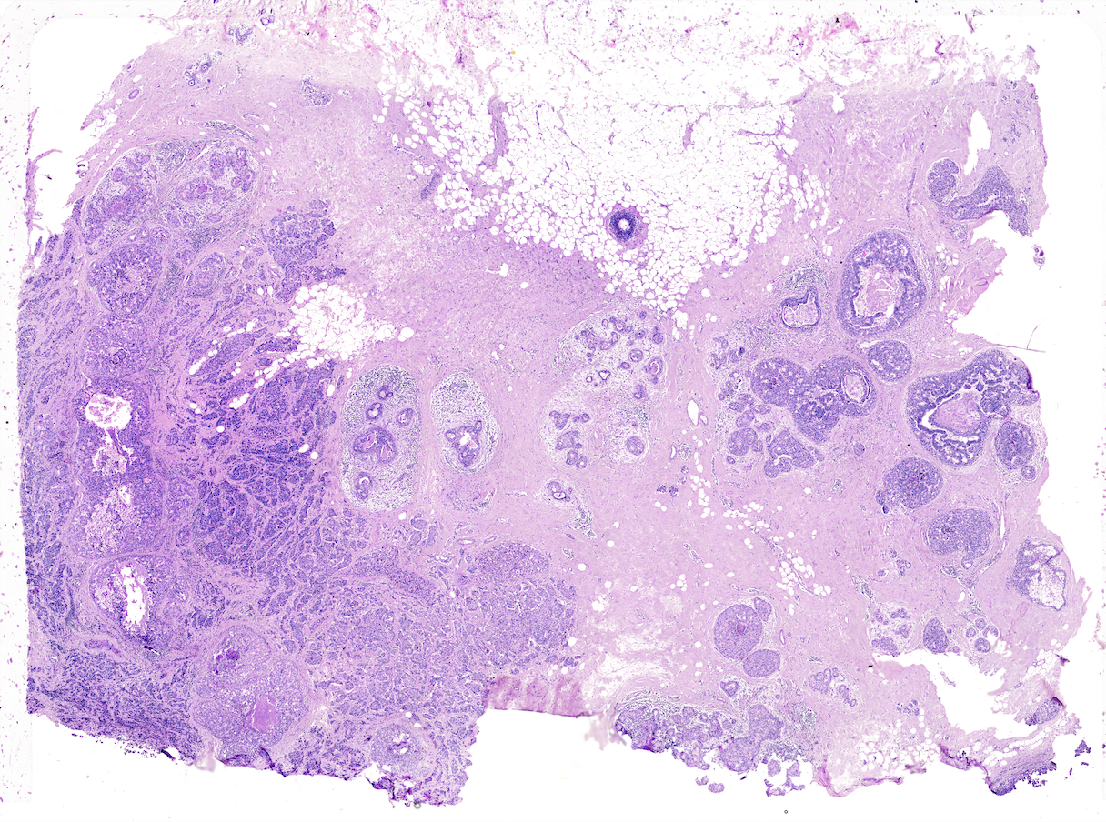
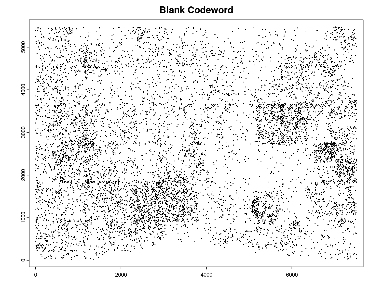
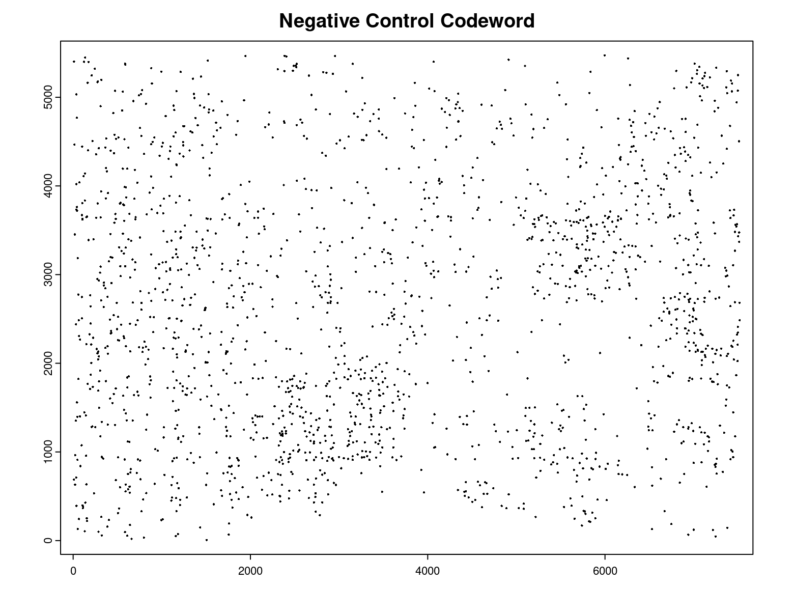
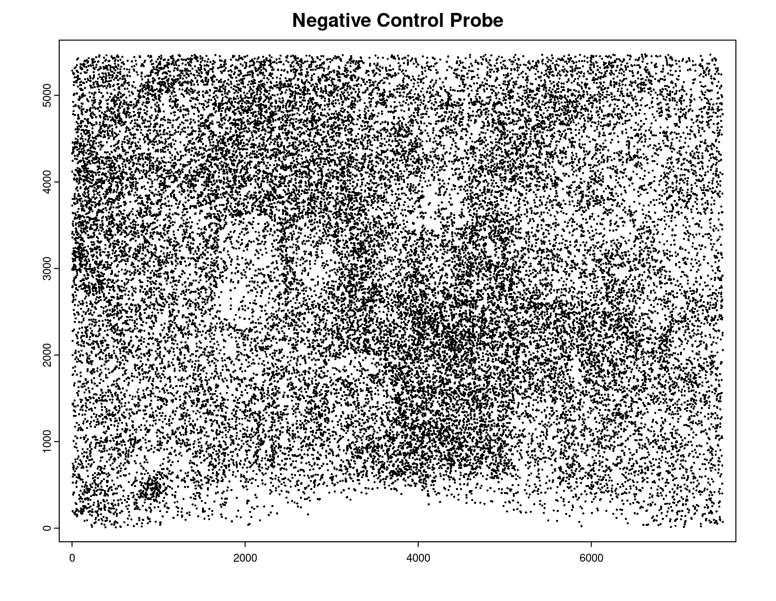
# Preview QC probe detections
plot(gpoints_list$`Blank Codeword`,
point_size = 0.3,
main = 'Blank Codeword')
plot(gpoints_list$`Negative Control Codeword`,
point_size = 0.3,
main = 'Negative Control Codeword')
plot(gpoints_list$`Negative Control Probe`,
point_size = 0.3,
main = 'Negative Control Probe')
# Preview two genes (slower)
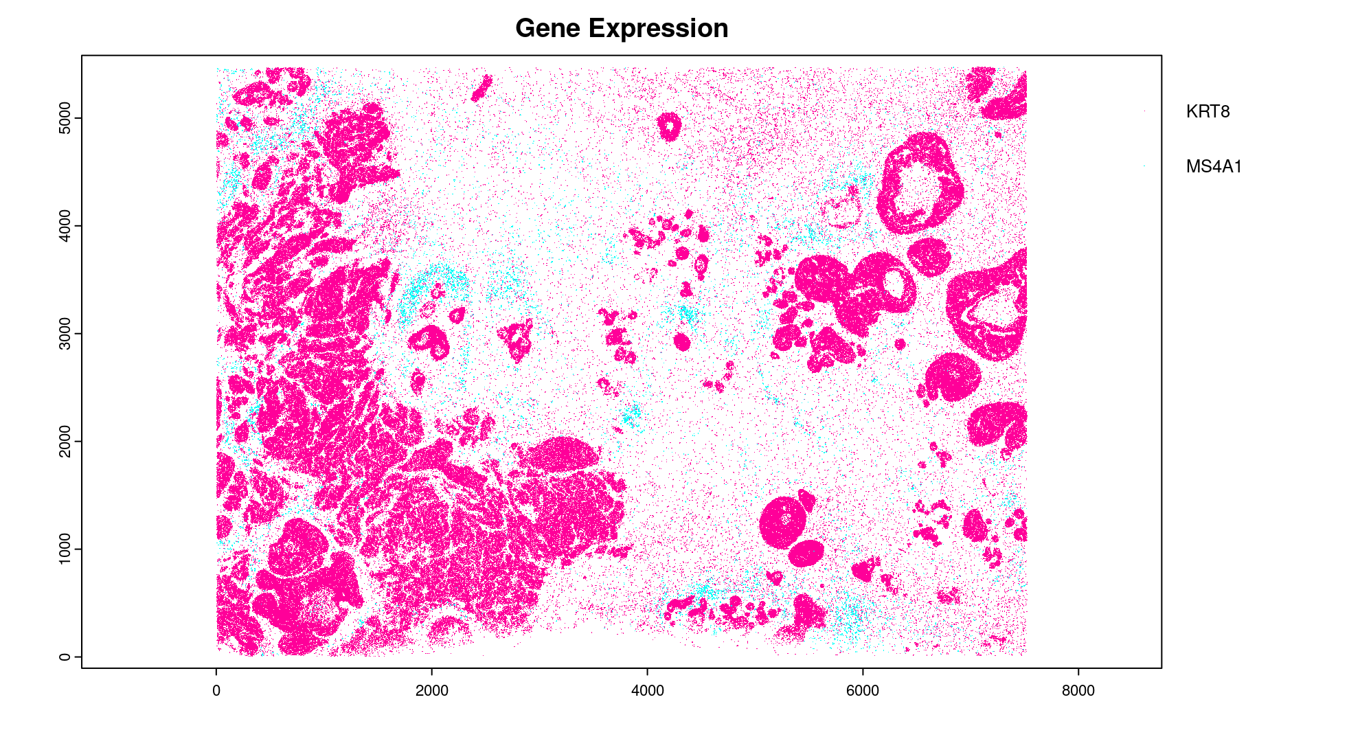
plot(gpoints_list$`Gene Expression`, # 77.843 sec elapsed
feats = c('KRT8', 'MS4A1'))
tx_dt_types$`Gene Expression`[feat_ID %in% c('KRT8', 'MS4A1'), table(feat_ID)]
# feat_ID
#   KRT8  MS4A1
# 530168  20875
7.1.2 Load polygon data#
Xenium output provides segmentation/cell boundary information in .csv.gz
files. These are represented within Giotto as giottoPolygon objects
and can also be directly plotted. This function also determines the
correct columns to use by looking for columns named 'poly_ID',
'x', and 'y'.
cellPoly_dt = data.table::fread(cell_bound_path)
nucPoly_dt = data.table::fread(nuc_bound_path)

data.table::setnames(cellPoly_dt,
                     old = c('cell_id', 'vertex_x', 'vertex_y'),
                     new = c('poly_ID', 'x', 'y'))
data.table::setnames(nucPoly_dt,
                     old = c('cell_id', 'vertex_x', 'vertex_y'),
                     new = c('poly_ID', 'x', 'y'))

gpoly_cells = createGiottoPolygonsFromDfr(segmdfr = cellPoly_dt,
                                          name = 'cell',
                                          calc_centroids = TRUE)
gpoly_nucs = createGiottoPolygonsFromDfr(segmdfr = nucPoly_dt,
                                         name = 'nucleus',
                                         calc_centroids = TRUE)
# Selecting col "poly_ID" as poly_ID column
# Selecting cols "x" and "y" as x and y respectively
# Selecting col "poly_ID" as poly_ID column
# Selecting cols "x" and "y" as x and y respectively
giottoPolygon objects can be directly plotted with plot(), but
the field of view here is so large that it would take a long time and
the details would be lost. Here, we will only plot the polygon centroids
for the cell nucleus polygons by accessing the calculated results within
the giottoPolygon’s spatVectorCentroids slot.
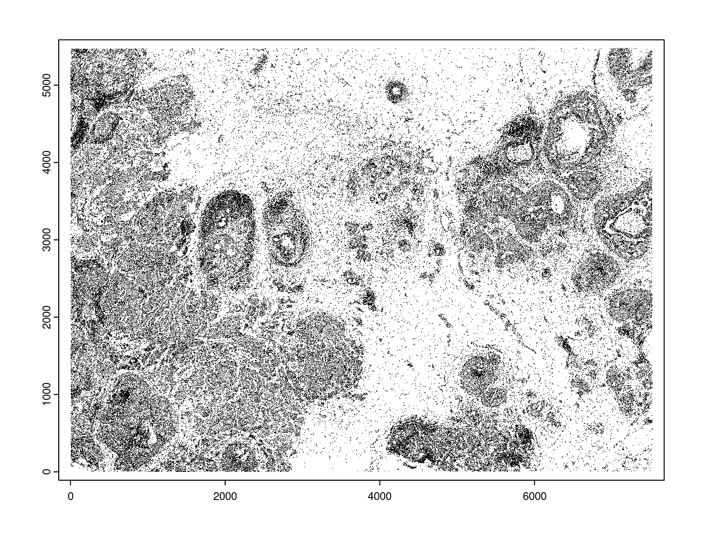
plot(x = gpoly_nucs, point_size = 0.1, type = 'centroid')
7.1.3 Create Giotto Object#
Now that both the feature data and the boundaries are loaded in, a subcellular Giotto object can be created.
xenium_gobj = createGiottoObjectSubcellular(
  gpoints = list(rna = gpoints_list$`Gene Expression`,
                 blank_code = gpoints_list$`Blank Codeword`,
                 neg_code = gpoints_list$`Negative Control Codeword`,
                 neg_probe = gpoints_list$`Negative Control Probe`),
  gpolygons = list(cell = gpoly_cells,
                   nucleus = gpoly_nucs),
  instructions = instrs
)
# polygonlist is a list with names
# [ cell ] Process polygon info...
# [ nucleus ] Process polygon info...
# pointslist is a named list
# [ rna ] Process point info...
# [ blank_code ] Process point info...
# [ neg_code ] Process point info...
# [ neg_probe ] Process point info...
8 Perform Bento Analysis#
8.1 Create Bento AnnData Object#
8.1.1 Subset Giotto Object First#
Large dataset may cause prolonged processing time for Bento.
subset_xenium_gobj <- subsetGiottoLocs(xenium_gobj, spat_unit='cell', feat_type='rna',
                                       x_max=200,x_min=0,y_max=200,y_min=0)
8.1.2 Create AnnData Object#
bento_adata <- createBentoAdata(subset_xenium_gobj,
                                env_to_use='/sc/arion/work/wangw32/conda-env/envs/giotto' # use the default value 'giotto_env' when you installed python dependencies automatically
                                )
# 14:27:41 --- INFO: Creating cell and nucleus segmentation dataframes
# 14:28:58 --- INFO: Batch information found in cell_shape, adding batch information to adata
8.2 Bento Analysis#
8.2.1 Load Python Modules#
bento_analysis_path <- system.file("python","python_bento_analysis.py",package="Giotto")
reticulate::source_python(bento_analysis_path)
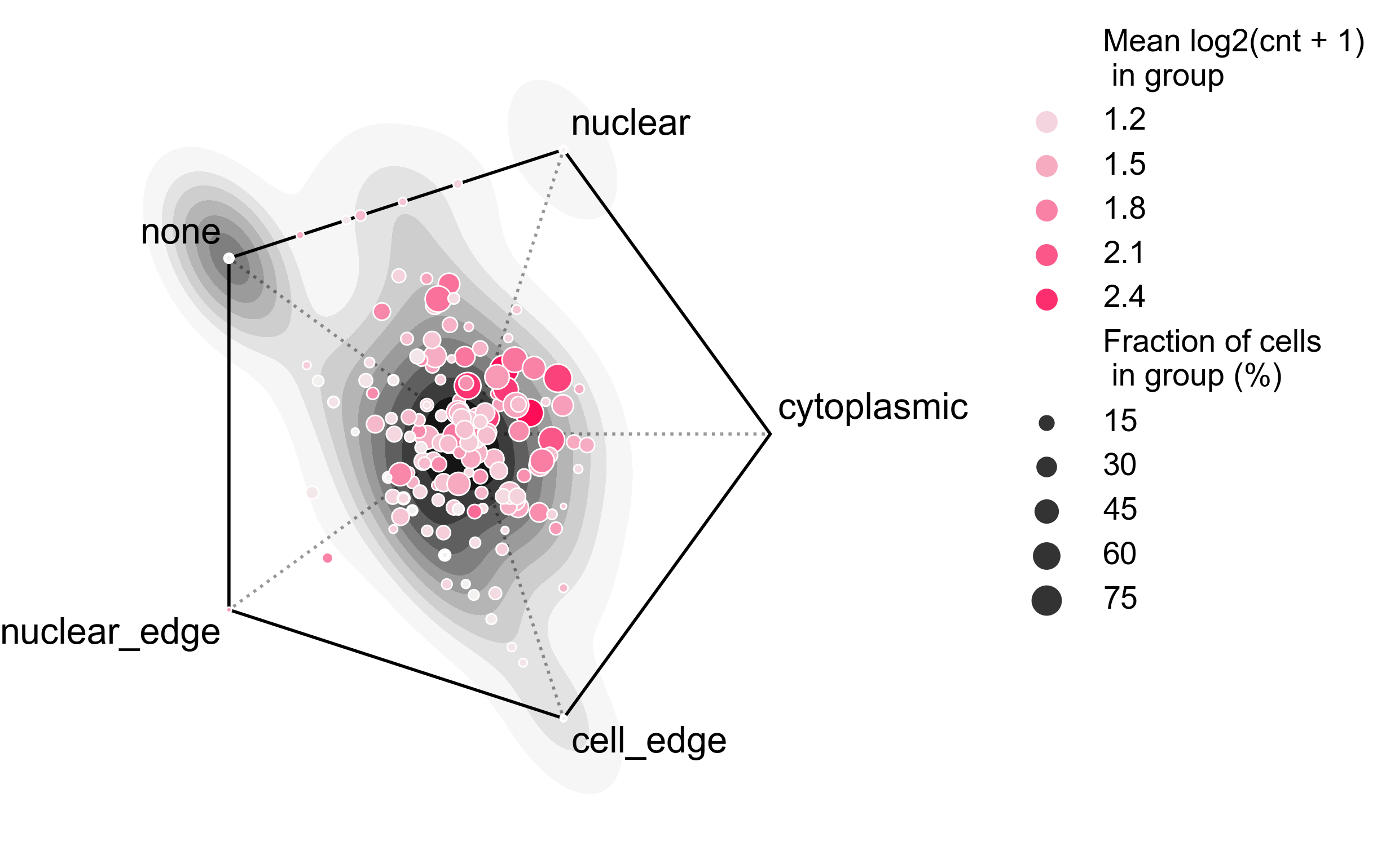
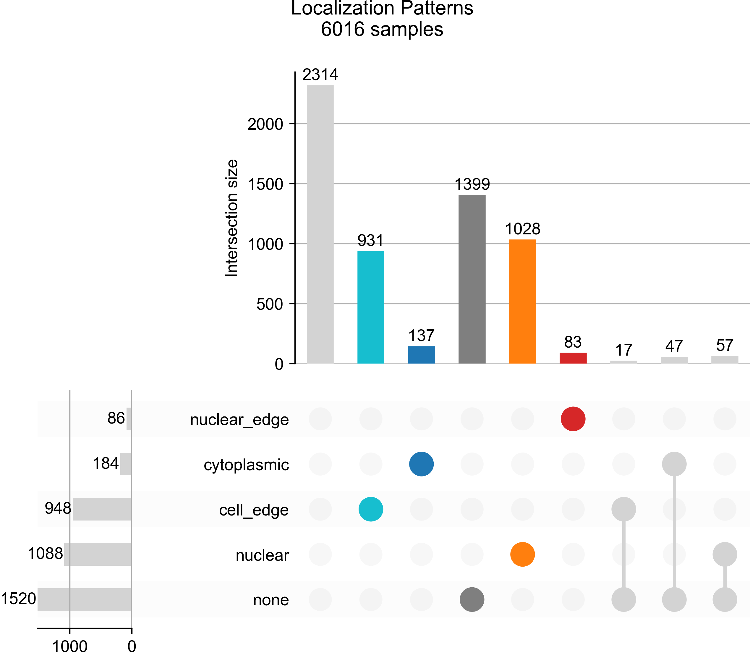
8.2.2 RNA Forest Analysis#
analysis_rna_forest(adata=bento_adata)
plot_rna_forest_analysis_results(adata=bento_adata,
                                 fname1='Bento_rna_forest_radvis.png',
                                 fname2='Bento_rna_forest_upset.png')
# Crunching shape features...
# AnnData object modified:
#     obs:
#         + cell_maxy, cell_raster, cell_area, cell_miny, cell_radius, cell_minx, cell_span, cell_maxx
#     uns:
#         + cell_raster
# Crunching point features...
# Saving results...
# Done.
# AnnData object modified:
#     obs:
#         + cell_maxy, cell_raster, cell_area, cell_miny, cell_radius, cell_minx, cell_span, cell_maxx
#     uns:
#         + cell_gene_features, cell_raster
# Crunching shape features...
# Crunching point features...
# Saving results...
# Done.
# AnnData object modified:
#     obs:
#         + cell_maxy, cell_raster, cell_area, cell_miny, cell_radius, cell_minx, cell_span, cell_maxx
#     uns:
#         + lp, cell_gene_features, cell_raster, lpp
# AnnData object modified:
#     uns:
#         + lp_stats

# Saved to Bento_rna_forest_radvis.png
# Saved to Bento_rna_forest_upset.png
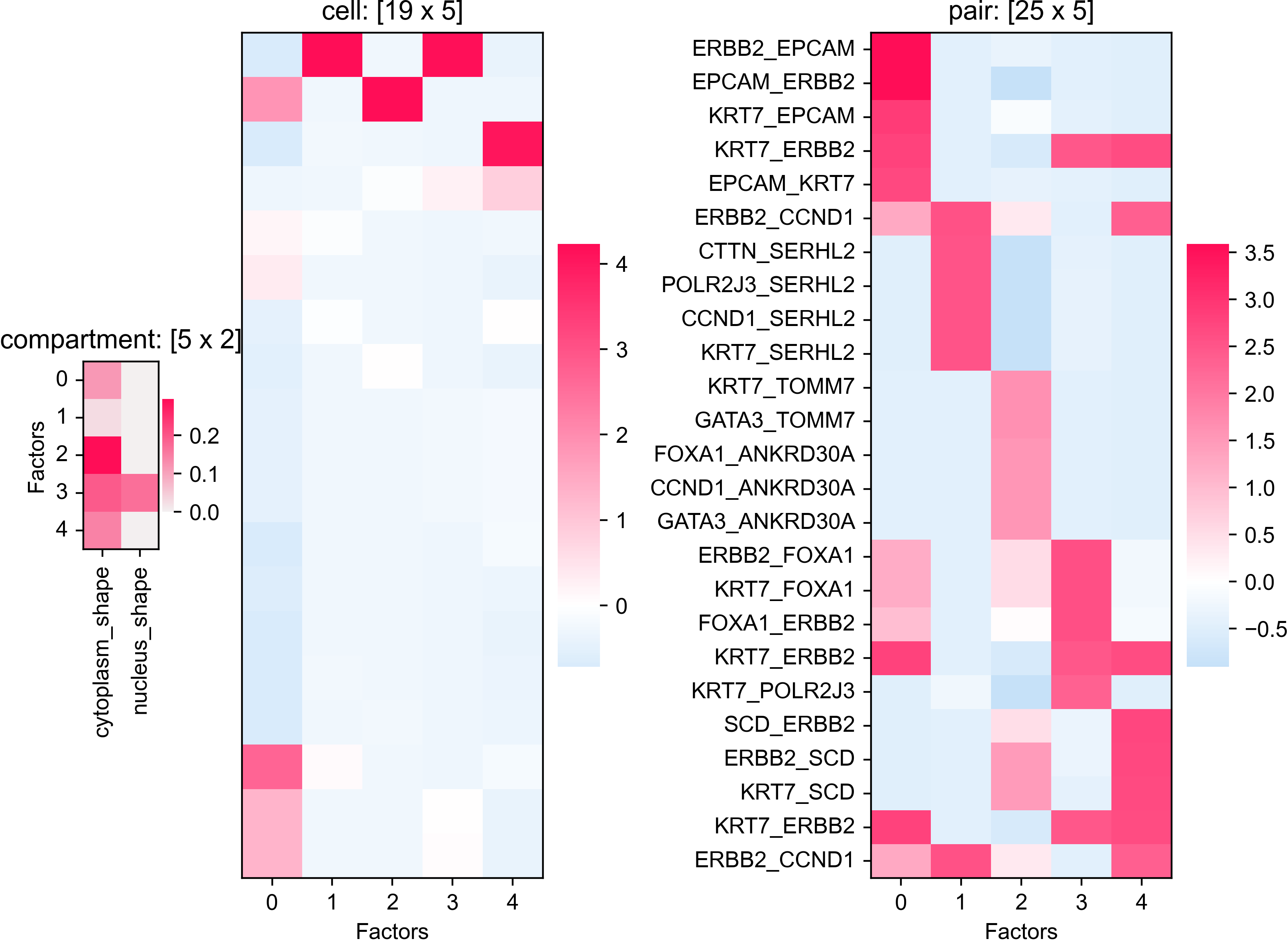
8.2.3 Colocalization Analysis#
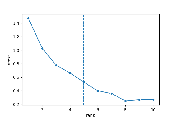
analysis_colocalization(adata=bento_adata, fname='Bento_colocalization_knee_pos.png', ranks=seq(10))
# Set the rank according output hint.
plot_colocalization_analysis_results(adata=bento_adata, rank=5, fname='Bento_colocalization.png')
# AnnData object modified:
#     uns:
#         + clq
# Preparing tensor...
# (2, 19, 156)
# :running: Decomposing tensor...
# 14:29:54 --- INFO: Knee found at rank 5
# 14:29:54 --- INFO: Saved to Bento_colocalization_knee_pos.png
# :heavy_check_mark: Done.
# AnnData object modified:
#     uns:
#         + tensor, tensor_names, tensor_labels, factors_error, factors

# Saved to Bento_colocalization.png
9 Session Info#
9.1 R Session Info#
sessionInfo()
# R version 4.2.3 (2023-03-15)
# Platform: x86_64-conda-linux-gnu (64-bit)
# Running under: Ubuntu 22.04.2 LTS
#
# Matrix products: default
# BLAS/LAPACK: /sc/arion/work/wangw32/conda-env/envs/giotto/lib/libopenblasp-r0.3.24.so
#
# locale:
#  [1] LC_CTYPE=en_US.UTF-8       LC_NUMERIC=C
#  [3] LC_TIME=en_US.UTF-8        LC_COLLATE=en_US.UTF-8
#  [5] LC_MONETARY=en_US.UTF-8    LC_MESSAGES=en_US.UTF-8
#  [7] LC_PAPER=en_US.UTF-8       LC_NAME=C
#  [9] LC_ADDRESS=C               LC_TELEPHONE=C
# [11] LC_MEASUREMENT=en_US.UTF-8 LC_IDENTIFICATION=C
#
# attached base packages:
# [1] stats     graphics  grDevices utils     datasets  methods   base
#
# other attached packages:
# [1] Giotto_4.0.0        GiottoVisuals_0.1.0 GiottoClass_0.1.0
# [4] GiottoUtils_0.1.0
#
# loaded via a namespace (and not attached):
#  [1] reticulate_1.34.0  tidyselect_1.2.0   terra_1.7-55       xfun_0.41
#  [5] sf_1.0-14          lattice_0.22-5     colorspace_2.1-0   vctrs_0.6.5
#  [9] generics_0.1.3     htmltools_0.5.7    yaml_2.3.7         utf8_1.2.4
# [13] rlang_1.1.2        e1071_1.7-13       R.oo_1.25.0        pillar_1.9.0
# [17] glue_1.6.2         withr_2.5.2        DBI_1.1.3          R.utils_2.12.3
# [21] rappdirs_0.3.3     bit64_4.0.5        lifecycle_1.0.4    stringr_1.5.1
# [25] munsell_0.5.0      gtable_0.3.4       R.methodsS3_1.8.2  codetools_0.2-19
# [29] evaluate_0.23      knitr_1.45         fastmap_1.1.1      class_7.3-22
# [33] parallel_4.2.3     fansi_1.0.5        Rcpp_1.0.11        KernSmooth_2.23-22
# [37] scales_1.3.0       backports_1.4.1    classInt_0.4-10    checkmate_2.3.1
# [41] jsonlite_1.8.7     bit_4.0.5          ggplot2_3.4.4      png_0.1-8
# [45] digest_0.6.33      stringi_1.8.2      dplyr_1.1.4        grid_4.2.3
# [49] scattermore_1.2    cli_3.6.1          tools_4.2.3        magrittr_2.0.3
# [53] proxy_0.4-27       tibble_3.2.1       colorRamp2_0.1.0   pkgconfig_2.0.3
# [57] Matrix_1.6-4       data.table_1.14.8  rmarkdown_2.25     rstudioapi_0.15.0
# [61] R6_2.5.1           units_0.8-5        compiler_4.2.3
9.2 Python Session Info#
python_session_info()
# -----
# anndata     0.9.2
# bento       2.0.1
# emoji       1.7.0
# geopandas   0.10.2
# kneed       0.8.5
# log         NA
# matplotlib  3.8.2
# minisom     NA
# numpy       1.26.2
# pandas      1.5.3
# rasterio    1.3.9
# scipy       1.11.4
# seaborn     0.12.2
# shapely     1.8.5.post1
# sklearn     1.3.2
# tqdm        4.66.1
# -----
# IPython             8.18.1
# PIL                 10.1.0
# adjustText          NA
# affine              2.4.0
# astropy             5.3.4
# asttokens           NA
# attr                23.1.0
# certifi             2023.11.17
# cffi                1.16.0
# click               8.1.7
# comm                0.1.4
# community           0.16
# contourpy           1.2.0
# cycler              0.12.1
# cython_runtime      NA
# dateutil            2.8.2
# decorator           5.1.1
# decoupler           1.5.0
# defusedxml          0.7.1
# erfa                2.0.1.1
# exceptiongroup      1.2.0
# executing           2.0.1
# fiona               1.9.5
# h5py                3.10.0
# igraph              0.11.3
# ipywidgets          8.1.1
# jedi                0.19.1
# joblib              1.3.2
# kiwisolver          1.4.5
# leidenalg           0.8.8
# llvmlite            0.41.1
# matplotlib_scalebar 0.8.1
# mpl_toolkits        NA
# natsort             8.4.0
# networkx            3.2.1
# numba               0.58.1
# packaging           23.2
# parso               0.8.3
# patsy               0.5.4
# pexpect             4.8.0
# pickleshare         0.7.5
# pkg_resources       NA
# prompt_toolkit      3.0.41
# psutil              5.9.5
# ptyprocess          0.7.0
# pure_eval           0.2.2
# pycparser           2.21
# pygeos              0.12.0
# pygments            2.17.2
# pyparsing           3.1.1
# pyproj              3.6.1
# pytz                2023.3.post1
# rpycall             NA
# rpytools            NA
# session_info        1.0.0
# setuptools          68.2.2
# six                 1.16.0
# sparse              0.13.0
# stack_data          0.6.2
# statsmodels         0.13.5
# tensorly            0.7.0
# texttable           1.7.0
# threadpoolctl       3.2.0
# traitlets           5.14.0
# typing_extensions   NA
# upsetplot           0.7.0
# wcwidth             0.2.12
# xgboost             1.4.2
# yaml                6.0.1
# zoneinfo            NA
# -----
# Python 3.10.13 | packaged by conda-forge | (main, Oct 26 2023, 18:20:51) [GCC 12.3.0]
# Linux-3.10.0-1160.el7.x86_64-x86_64-with-glibc2.35
# -----
# Session information updated at 2023-12-19 14:29