Mouse Visium Brain#
- Date:
2022-09-16
# Ensure Giotto Suite is installed.
if(!"Giotto" %in% installed.packages()) {
  devtools::install_github("drieslab/Giotto@suite")
}

# Ensure GiottoData, a small, helper module for tutorials, is installed.
if(!"GiottoData" %in% installed.packages()) {
  devtools::install_github("drieslab/GiottoData")
}
library(Giotto)
# Ensure the Python environment for Giotto has been installed.
genv_exists = checkGiottoEnvironment()
if(!genv_exists){
  # The following command need only be run once to install the Giotto environment.
  installGiottoEnvironment()
}
Set up Giotto Environment#
library(Giotto)
library(GiottoData)

# 1. set working directory
results_folder = 'path/to/result'

# Optional: Specify a path to a Python executable within a conda or miniconda
# environment. If set to NULL (default), the Python executable within the previously
# installed Giotto environment will be used.
my_python_path = NULL # alternatively, "/local/python/path/python" if desired.

# 3. Create Giotto Instructions
instrs = createGiottoInstructions(save_dir = results_folder,
                                  save_plot = TRUE,
                                  show_plot = FALSE,
                                  python_path = my_python_path)
Dataset explanation#
10X genomics recently launched a new platform to obtain spatial expression data using a Visium Spatial Gene Expression slide.
The Visium brain data to run this tutorial can be found here
Visium technology:
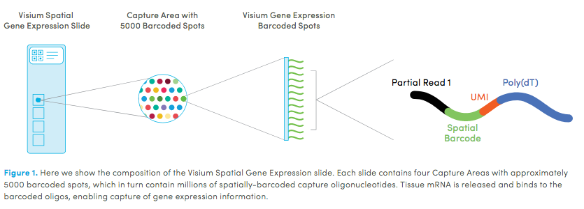
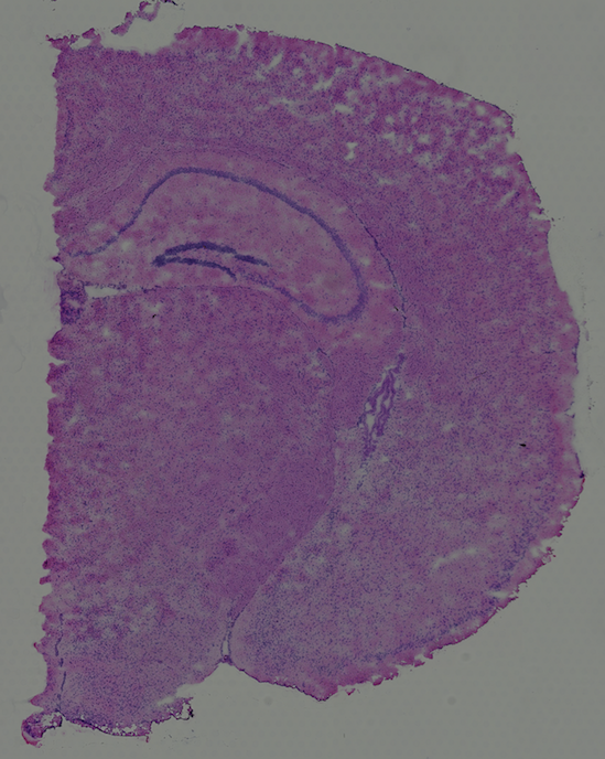
High resolution png from original tissue:
Part 1: Create Giotto Visium Object and visualize#
## provide path to visium folder
data_path = '/path/to/Brain_data/'
## directly from visium folder
visium_brain = createGiottoVisiumObject(visium_dir = data_path,
expr_data = 'raw',
png_name = 'tissue_lowres_image.png',
gene_column_index = 2,
instructions = instrs)
## show associated images with giotto object
showGiottoImageNames(visium_brain) # "image" is the default name
## check metadata
pDataDT(visium_brain)
## show plot
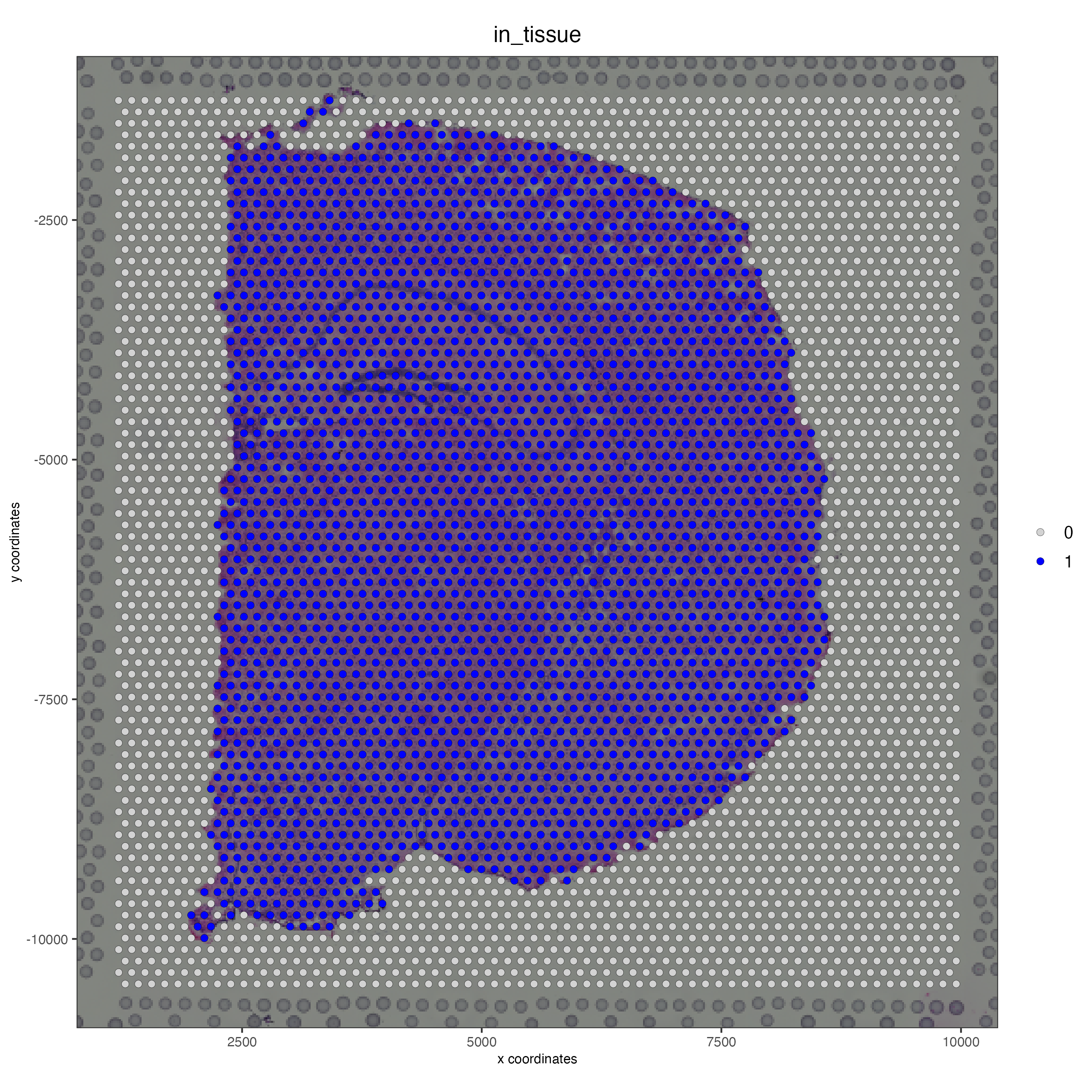
spatPlot2D(gobject = visium_brain, cell_color = 'in_tissue', point_size = 2,
cell_color_code = c('0' = 'lightgrey', '1' = 'blue'),
show_image = T, image_name = 'image')
Part 2: Process Giotto Visium Object#
## subset on spots that were covered by tissue
metadata = pDataDT(visium_brain)
in_tissue_barcodes = metadata[in_tissue == 1]$cell_ID
visium_brain = subsetGiotto(visium_brain, cell_ids = in_tissue_barcodes)
## filter
visium_brain <- filterGiotto(gobject = visium_brain,
expression_threshold = 1,
feat_det_in_min_cells = 50,
min_det_feats_per_cell = 1000,
expression_values = c('raw'),
verbose = T)
## normalize
visium_brain <- normalizeGiotto(gobject = visium_brain, scalefactor = 6000, verbose = T)
## add gene & cell statistics
visium_brain <- addStatistics(gobject = visium_brain)
## visualize
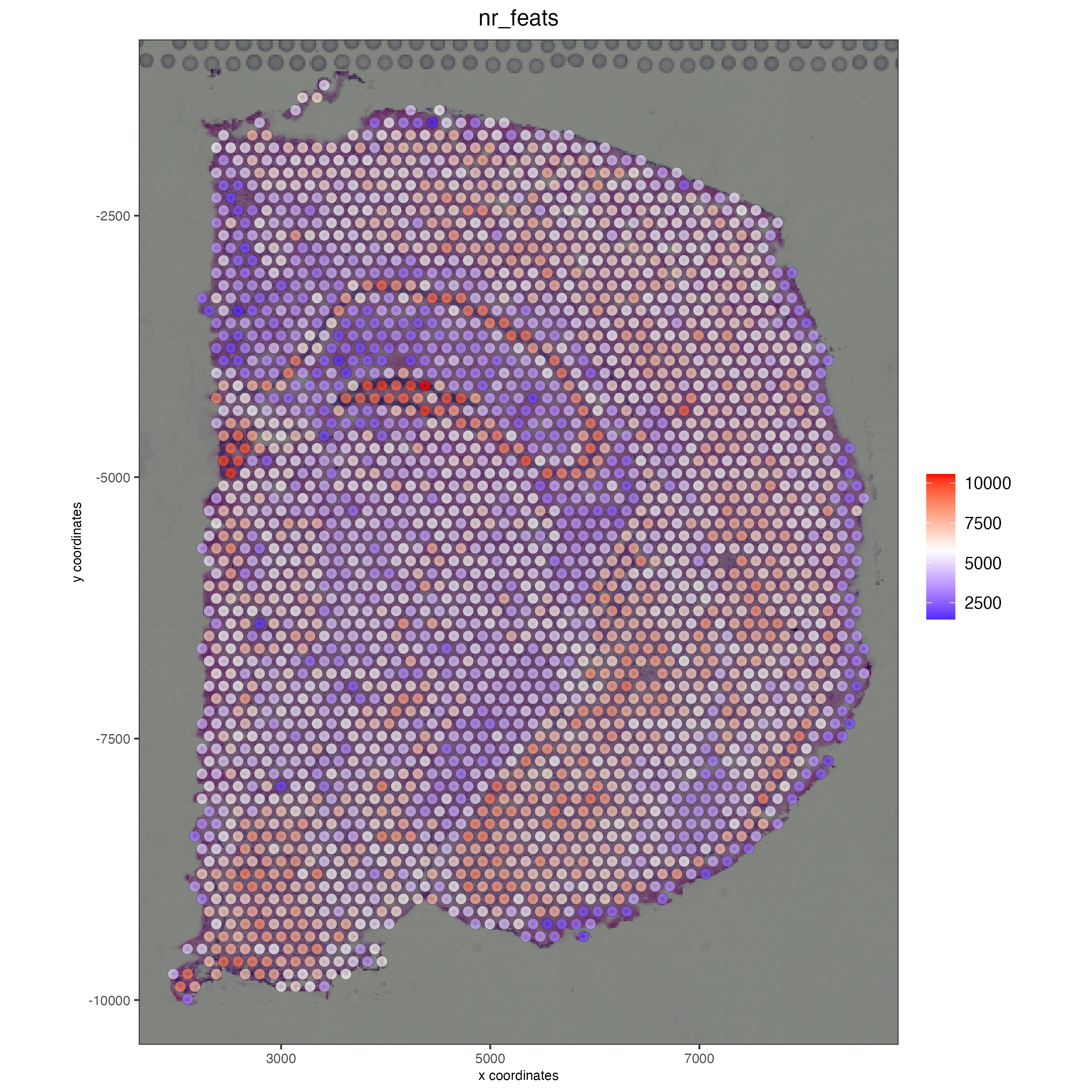
spatPlot2D(gobject = visium_brain, show_image = T, point_alpha = 0.7,
cell_color = 'nr_feats', color_as_factor = F)
Part 3: Dimention Reduction#
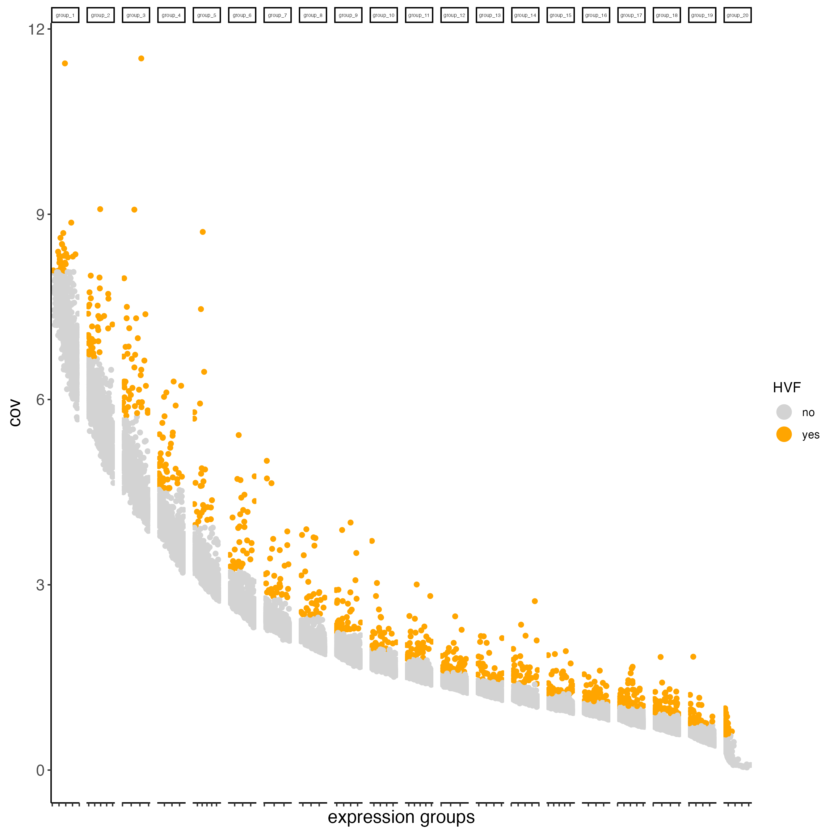
## highly variable features / genes (HVF)
visium_brain <- calculateHVF(gobject = visium_brain, save_plot = TRUE)
## run PCA on expression values (default)
gene_metadata = fDataDT(visium_brain)
featgenes = gene_metadata[hvf == 'yes' & perc_cells > 3 & mean_expr_det > 0.4]$feat_ID
## run PCA on expression values (default)
visium_brain <- runPCA(gobject = visium_brain,
feats_to_use = featgenes)
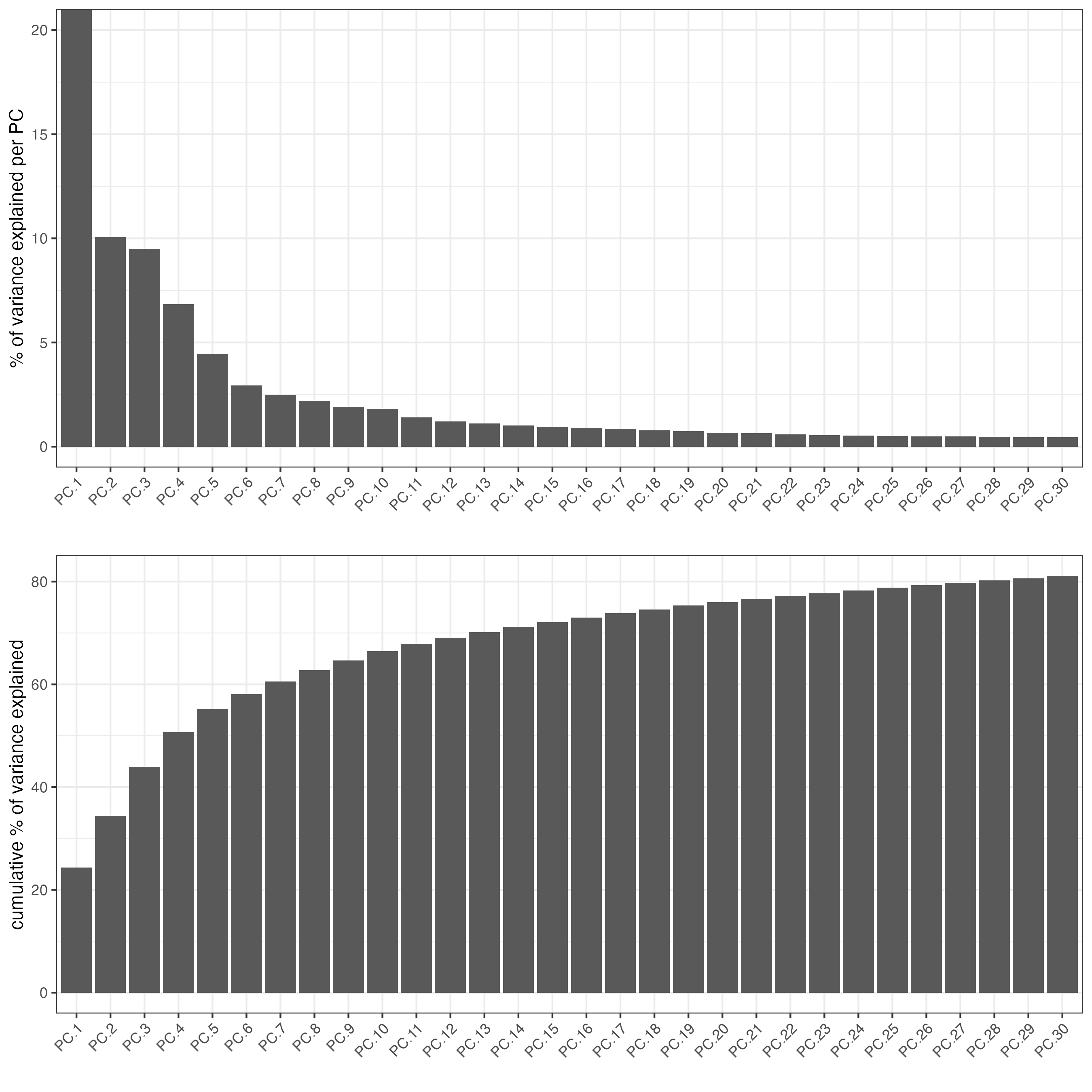
screePlot(visium_brain, ncp = 30)
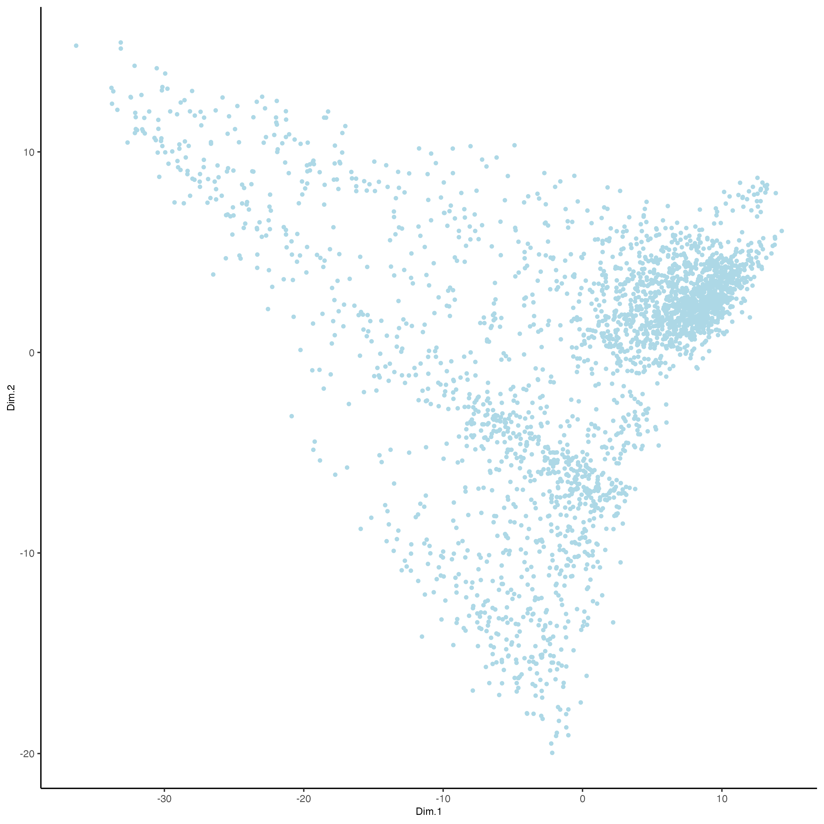
dimPlot2D(gobject = visium_brain,dim_reduction_to_use = "pca")
## run UMAP and tSNE on PCA space (default)
visium_brain <- runUMAP(visium_brain, dimensions_to_use = 1:10)
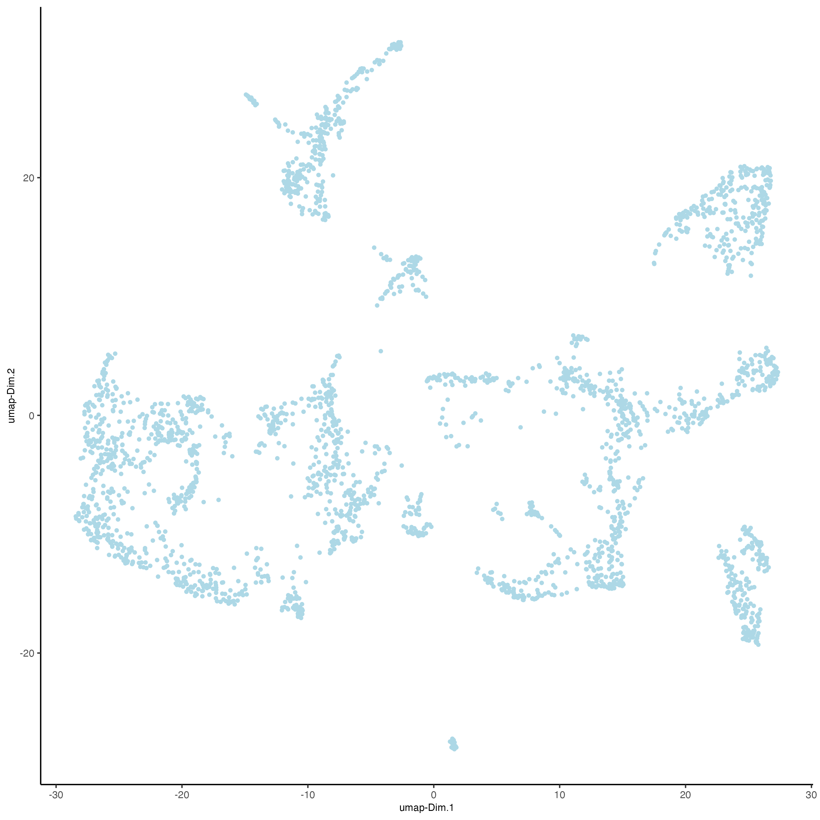
plotUMAP(gobject = visium_brain)
visium_brain <- runtSNE(visium_brain, dimensions_to_use = 1:10)
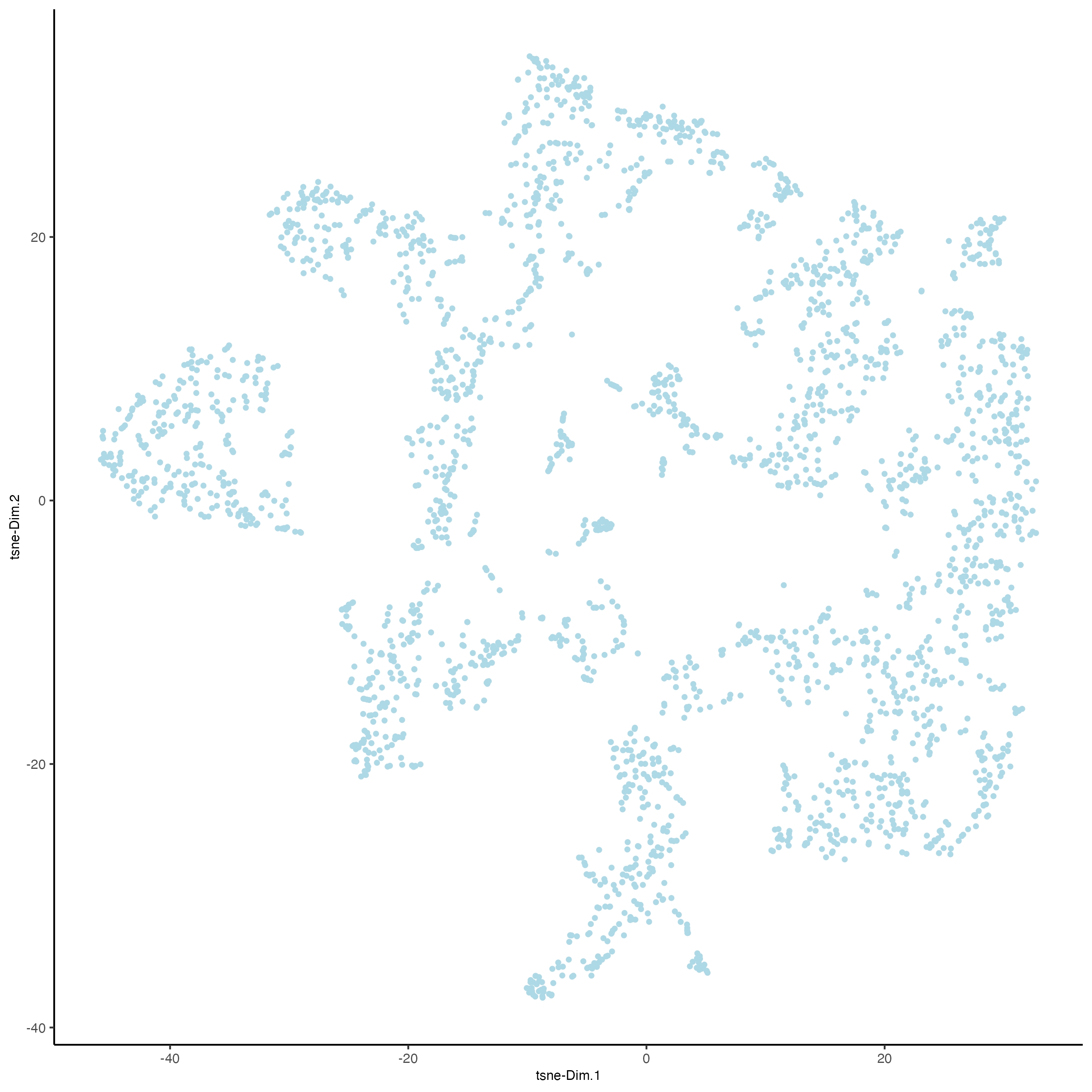
plotTSNE(gobject = visium_brain)
Part 4: Cluster#
## sNN network (default)
visium_brain <- createNearestNetwork(gobject = visium_brain, dimensions_to_use = 1:10, k = 15)
## Leiden clustering
visium_brain <- doLeidenCluster(gobject = visium_brain, resolution = 0.4, n_iterations = 1000)
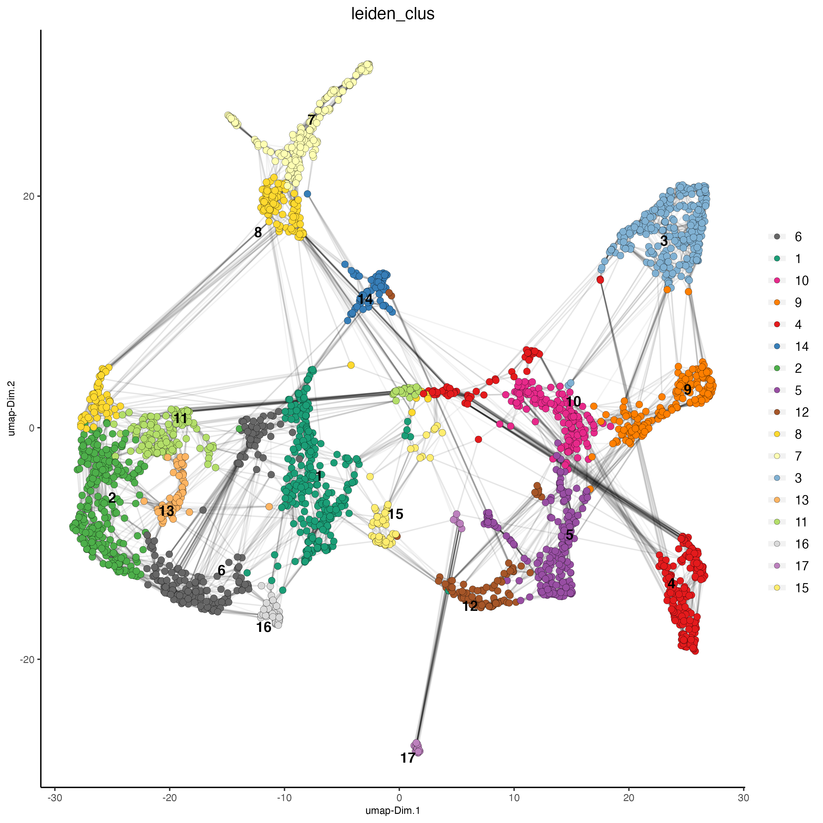
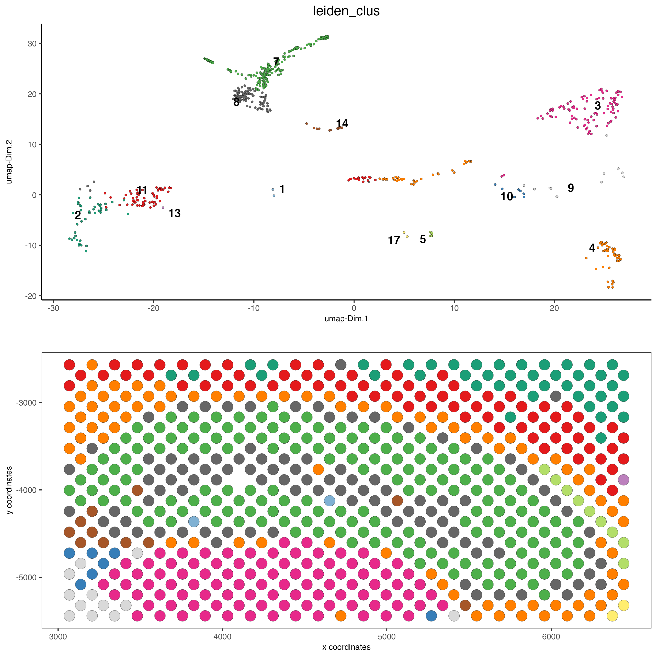
plotUMAP(gobject = visium_brain,
cell_color = 'leiden_clus', show_NN_network = T, point_size = 2.5)
# spatial and dimension plots
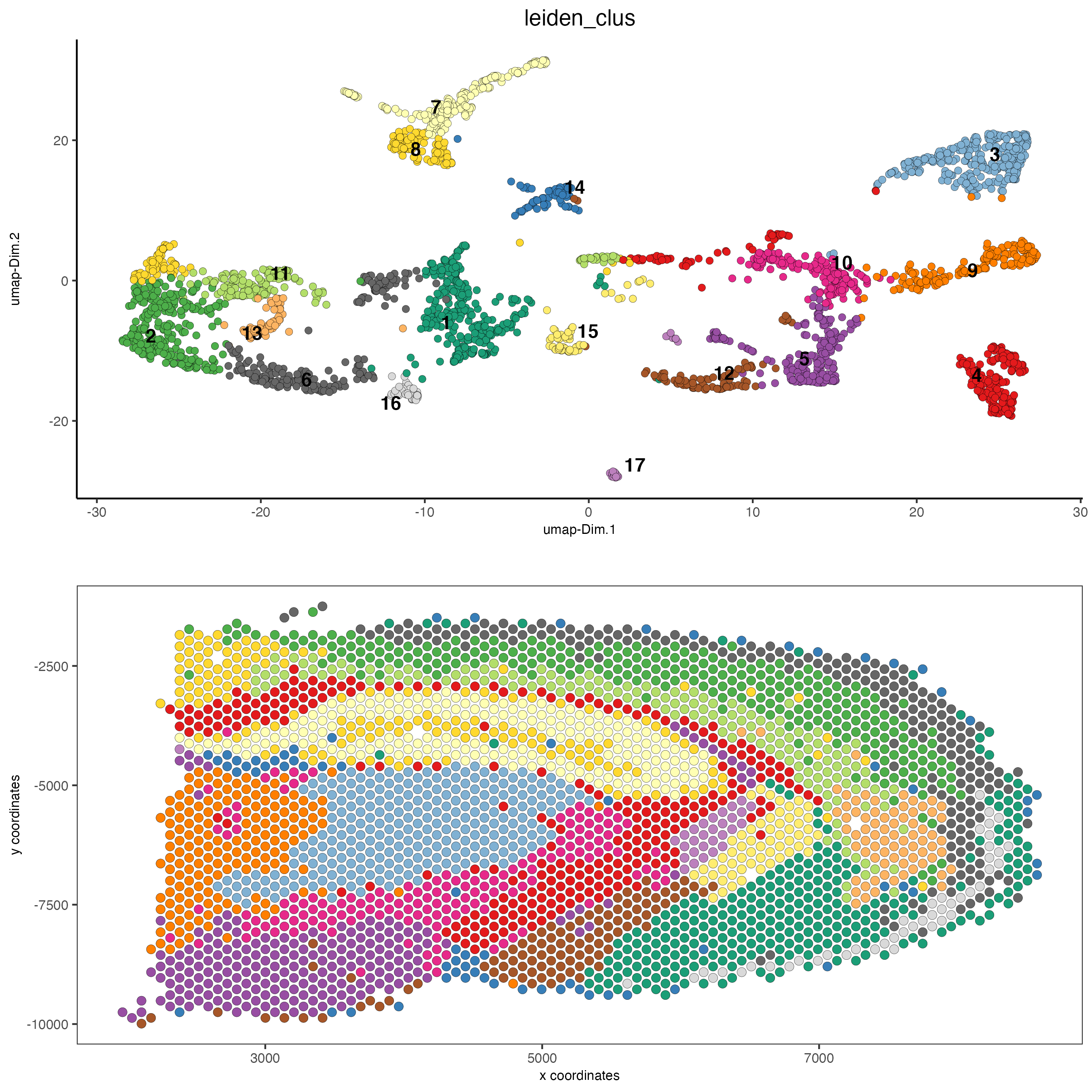
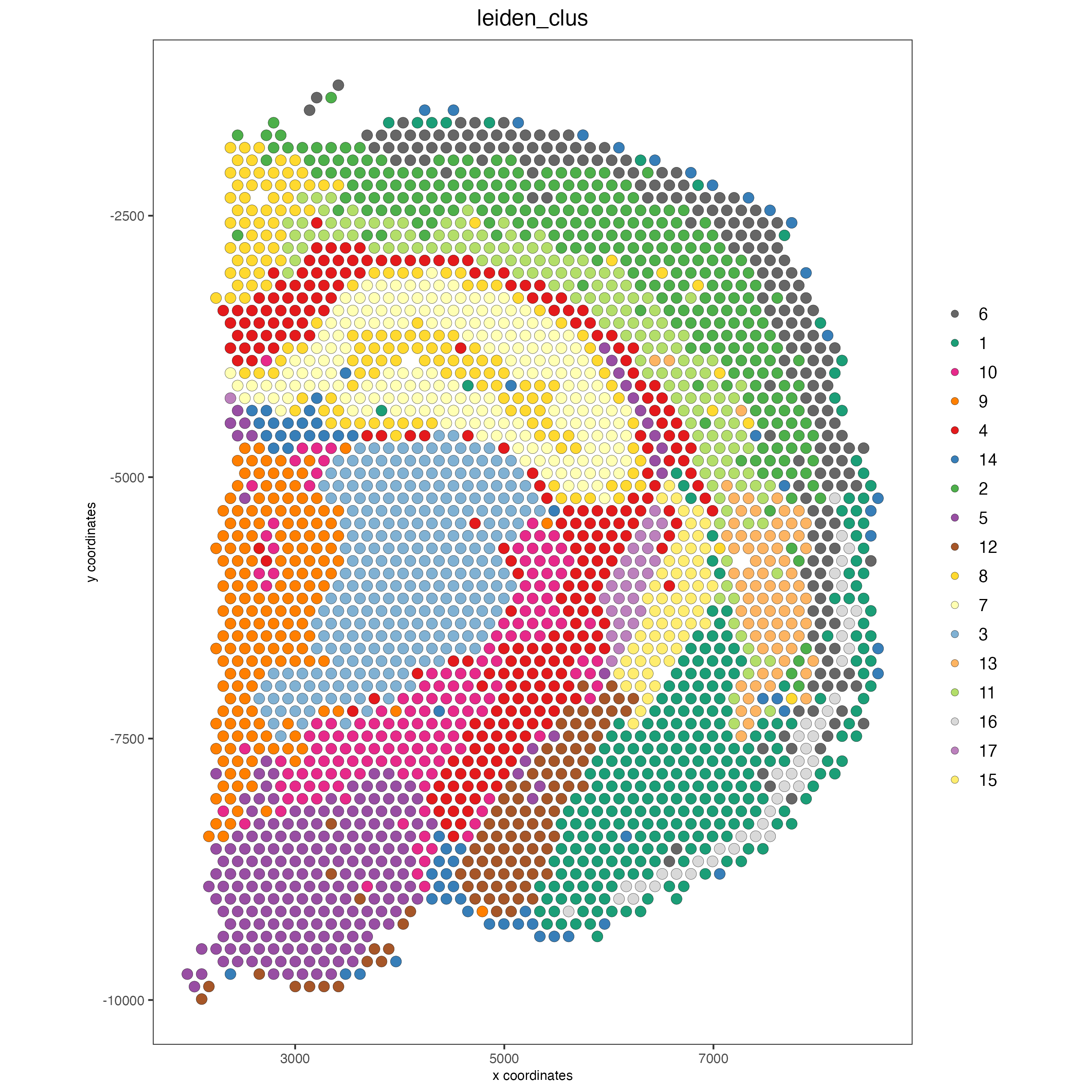
spatDimPlot(gobject = visium_brain, cell_color = 'leiden_clus',
dim_point_size = 2, spat_point_size = 2.5)
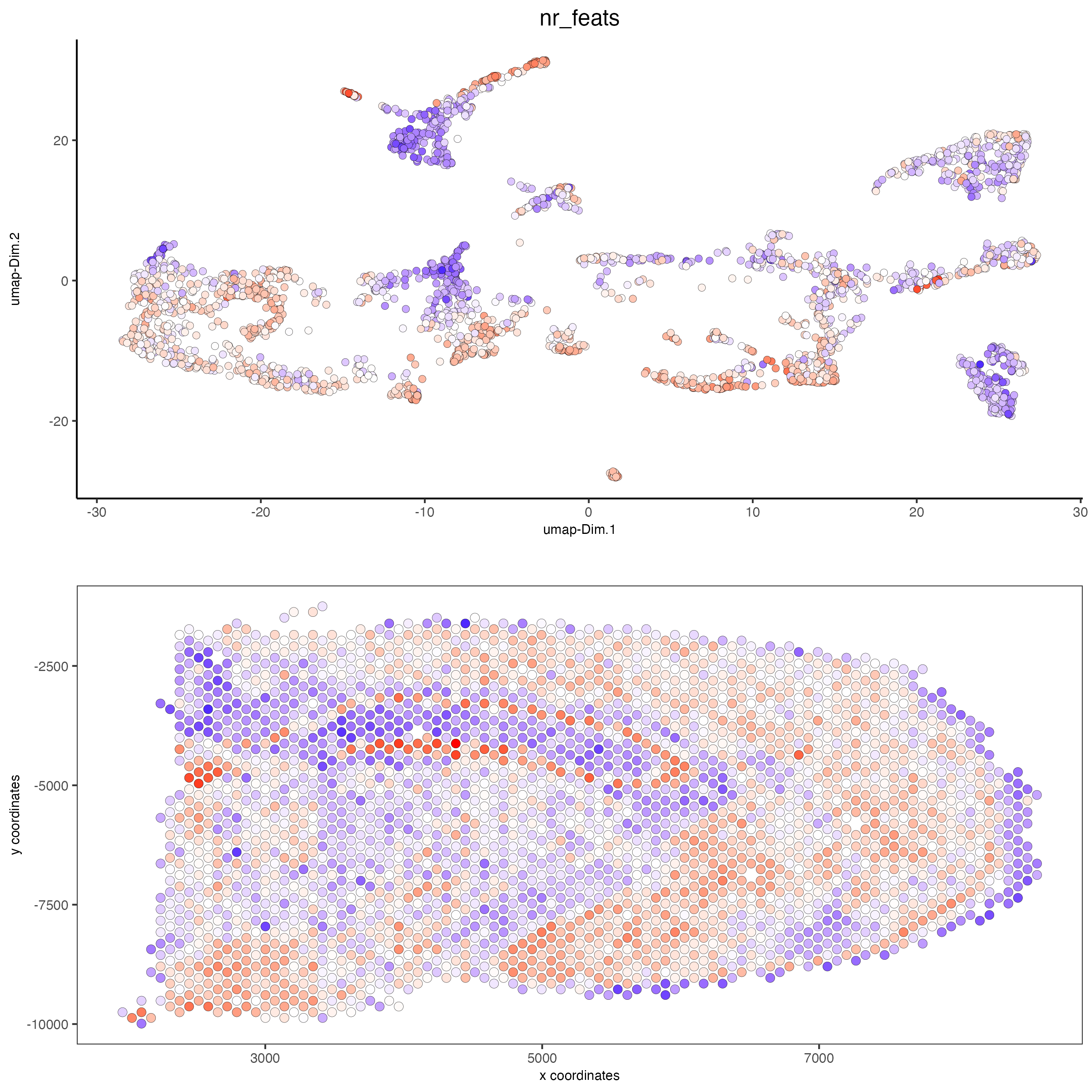
spatDimPlot(gobject = visium_brain, cell_color = 'nr_feats', color_as_factor = F,
            dim_point_size = 2, spat_point_size = 2.5)
# dimension plots grouped by cluster
spatPlot2D(visium_brain, cell_color = 'leiden_clus',
           coord_fix_ratio = 1)
Plot with group by:
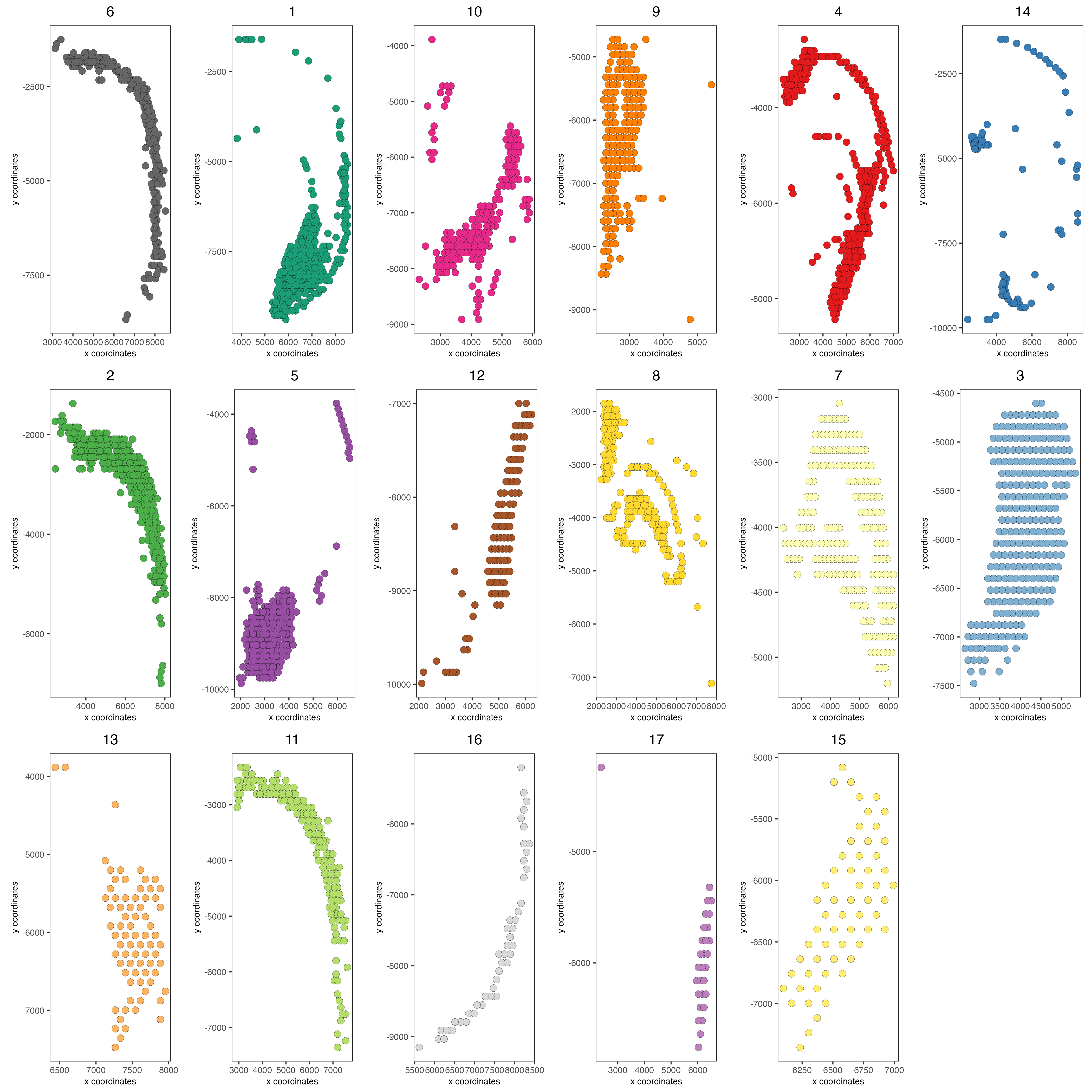
spatPlot2D(visium_brain, cell_color = 'leiden_clus',
           group_by = 'leiden_clus', coord_fix_ratio = 1,
           cow_n_col = 6, show_legend = F,
           save_param = list(base_width = 14, base_height = 14))
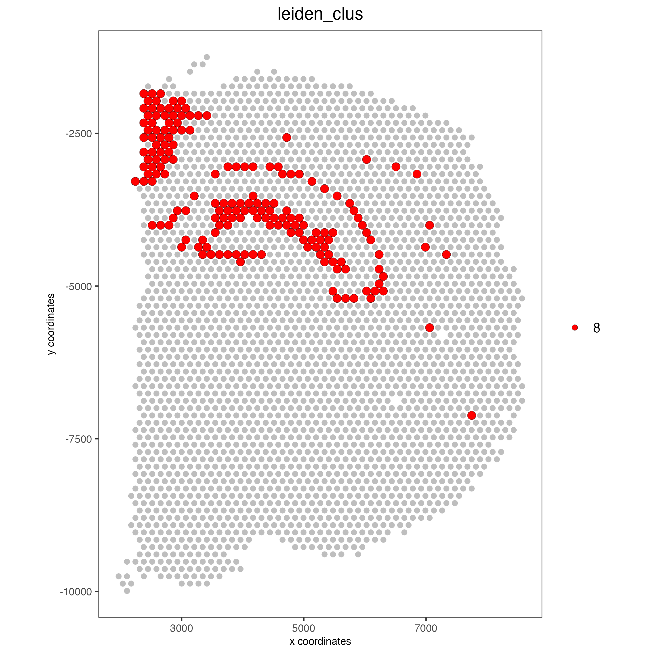
Highlight one or more groups:
spatPlot2D(visium_brain, cell_color = 'leiden_clus',
           select_cell_groups = '8', coord_fix_ratio = 1, show_other_cells = TRUE,
           cell_color_code = c('8' = 'red'), other_cell_color = "grey", other_point_size = 1.5,
           save_param = list(base_width = 7, base_height = 7))
Part 5: subset data#
# create and show subset
DG_subset = subsetGiottoLocs(visium_brain,
                             x_max = 6500, x_min = 3000,
                             y_max = -2500, y_min = -5500,
                             return_gobject = TRUE)

spatDimPlot(gobject = DG_subset,
            cell_color = 'leiden_clus', spat_point_size = 5)
Part 6: marker gene detection for clusters#
## ------------------ ##
## Gini markers
gini_markers_subclusters = findMarkers_one_vs_all(gobject = visium_brain,
method = 'gini',
expression_values = 'normalized',
cluster_column = 'leiden_clus',
min_feats = 20,
min_expr_gini_score = 0.5,
min_det_gini_score = 0.5)
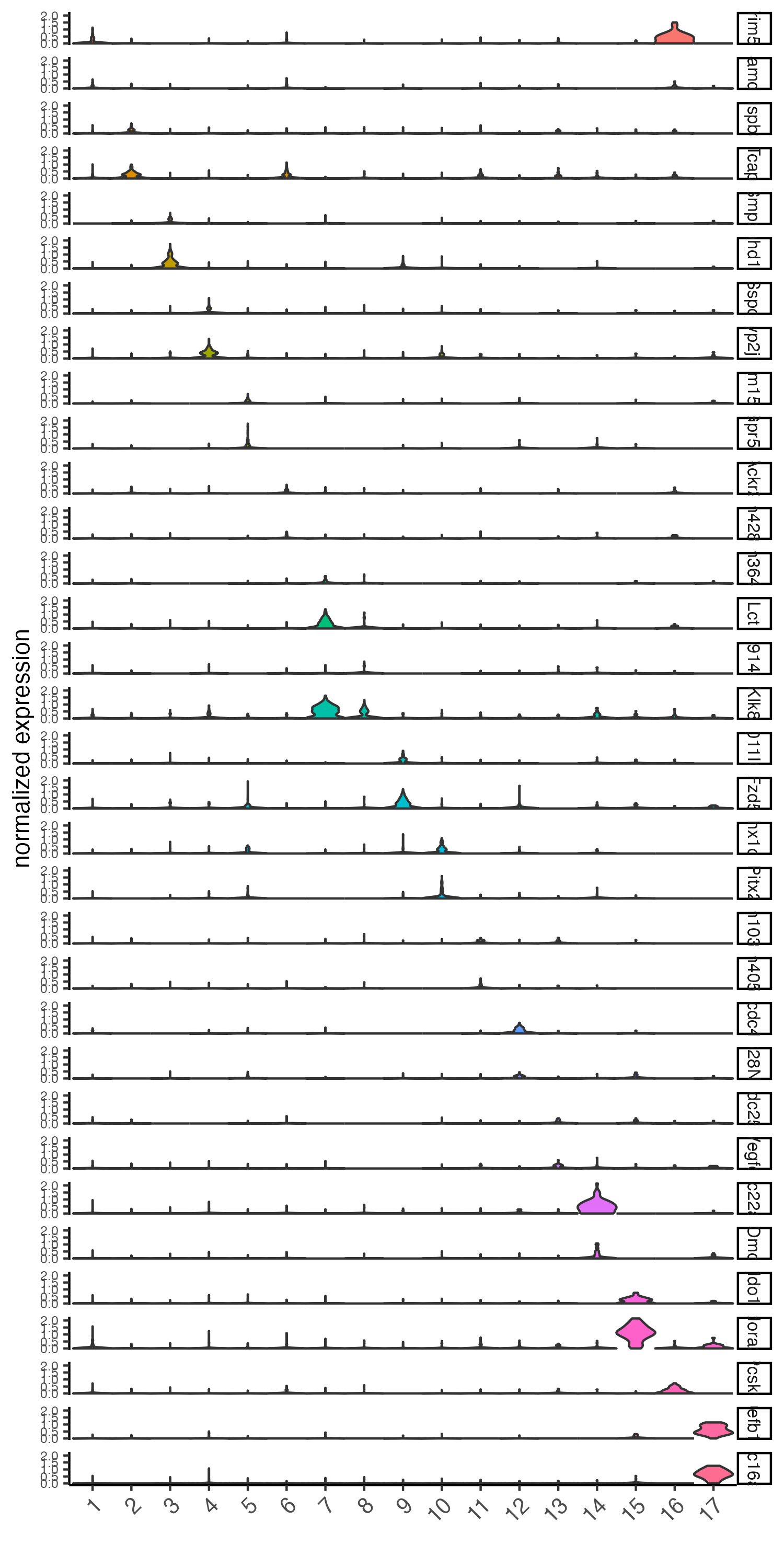
topgenes_gini = gini_markers_subclusters[, head(.SD, 2), by = 'cluster']$feats
# violinplot
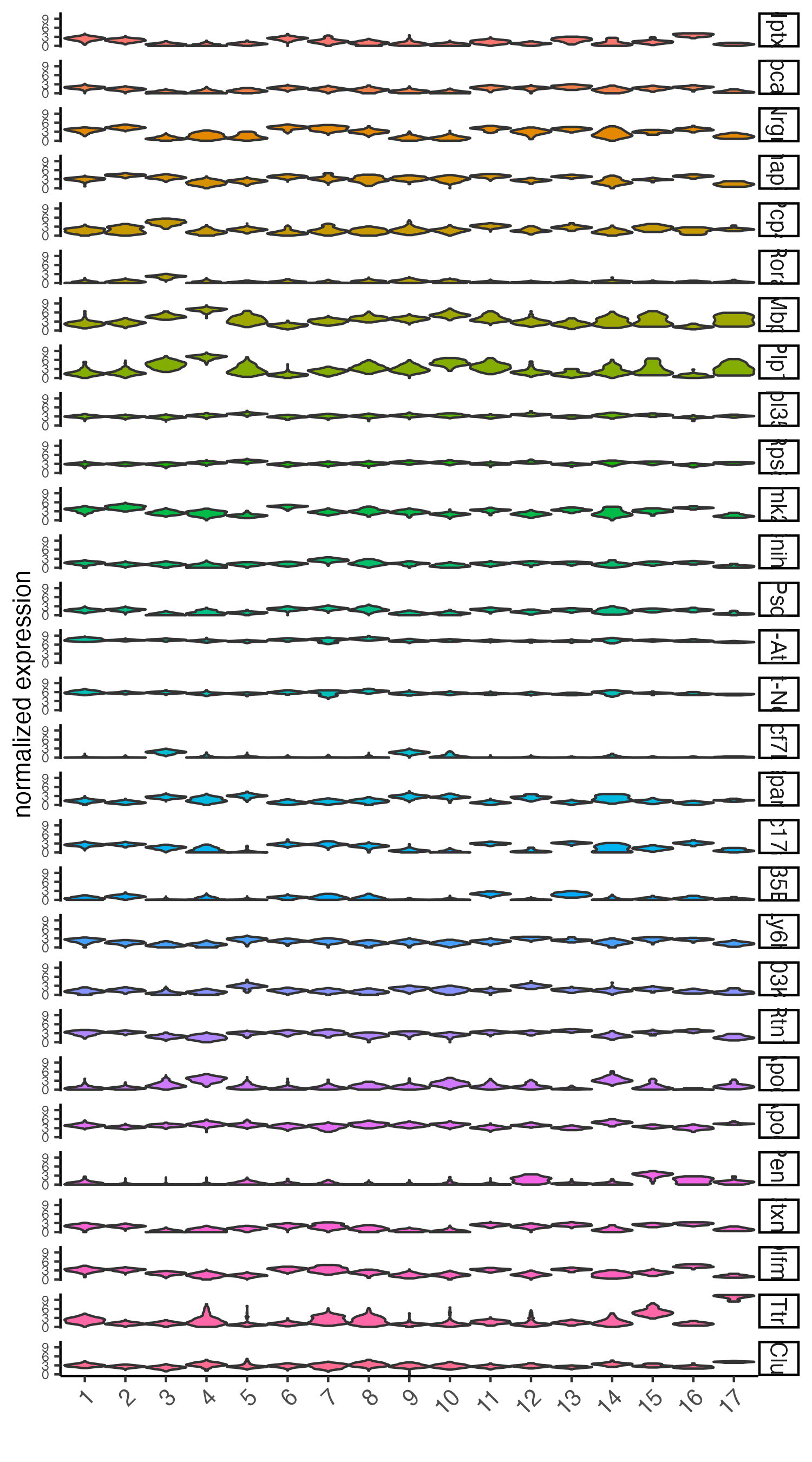
violinPlot(visium_brain, feats = unique(topgenes_gini), cluster_column = 'leiden_clus',
strip_text = 8, strip_position = 'right',
save_param = list(base_width = 5, base_height = 10))
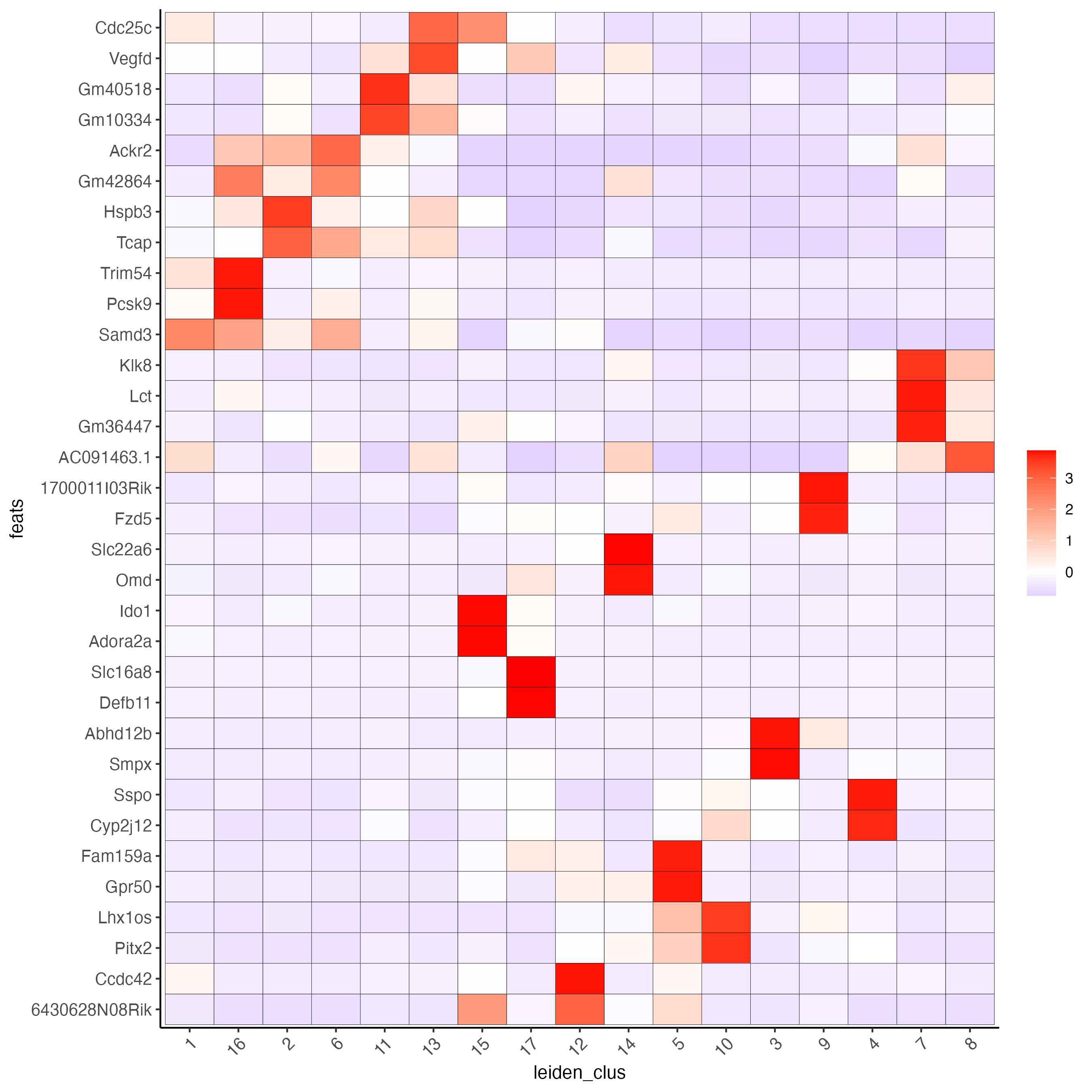
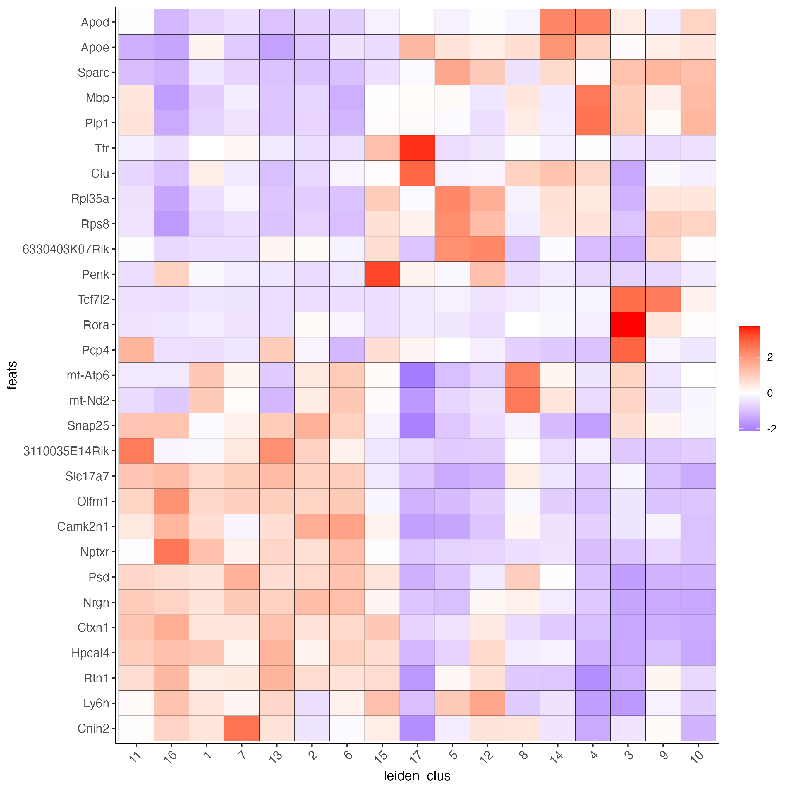
# cluster heatmap
plotMetaDataHeatmap(visium_brain, selected_feats = unique(topgenes_gini),
                    metadata_cols = c('leiden_clus'),
                    x_text_size = 10, y_text_size = 10)
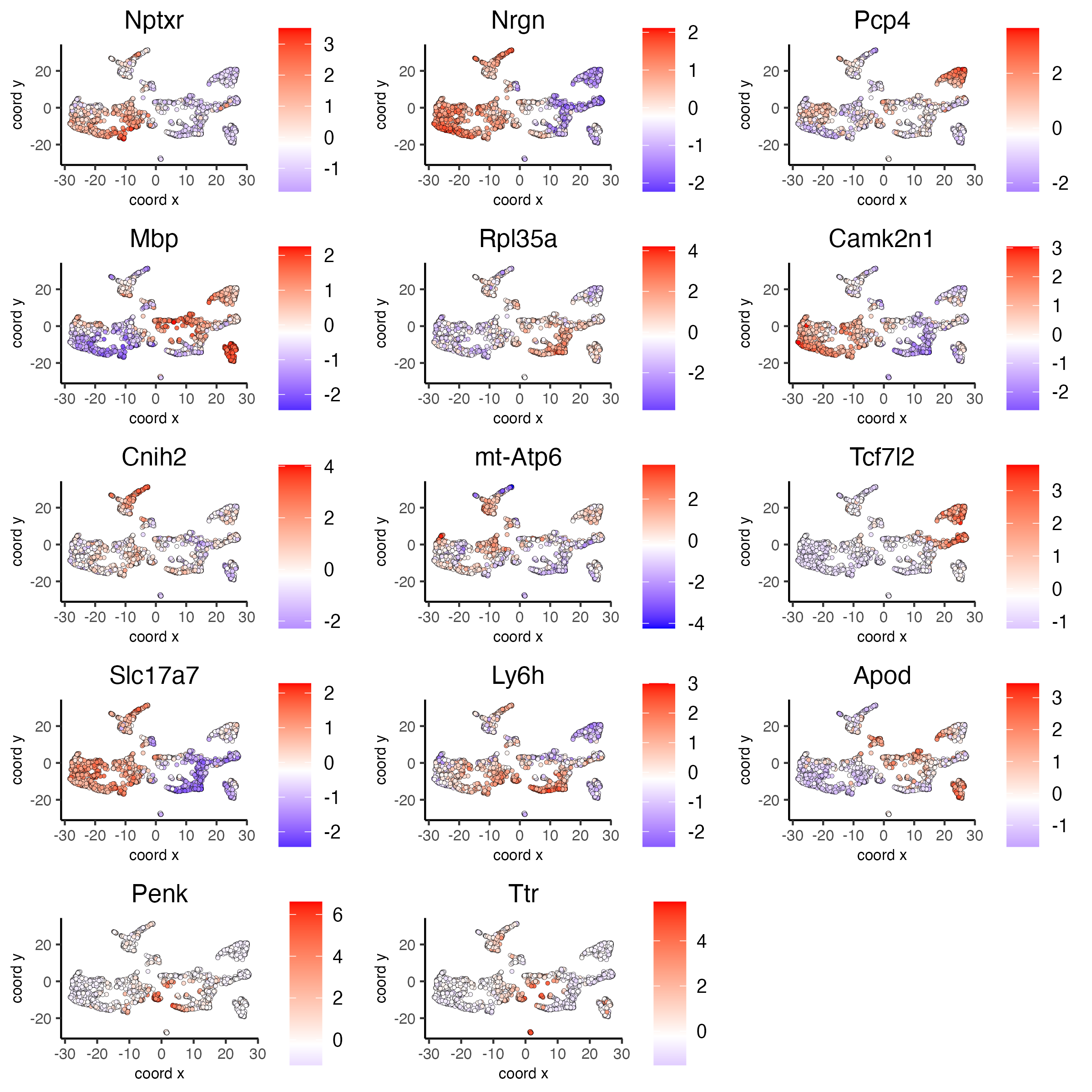
# umap plots
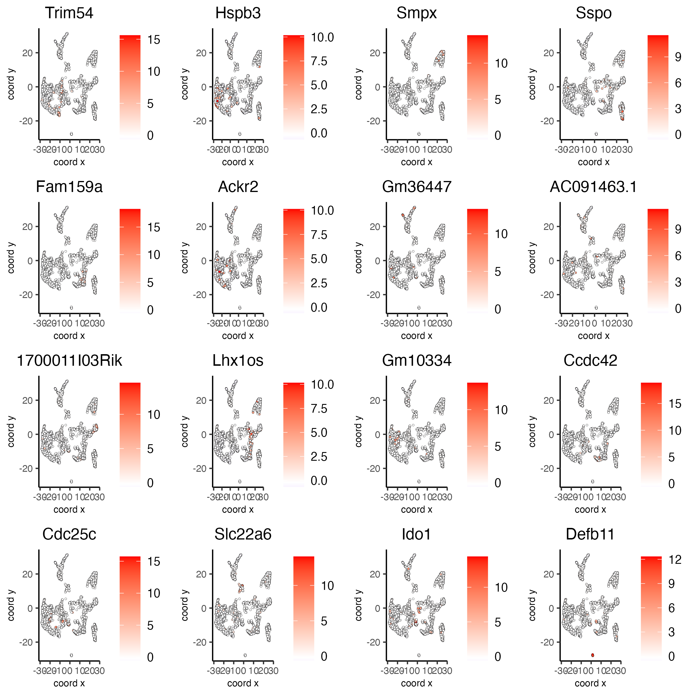
dimFeatPlot2D(visium_brain, expression_values = 'scaled',
feats = gini_markers_subclusters[, head(.SD, 1), by = 'cluster']$feats,
cow_n_col = 4, point_size = 0.75,
save_param = list(base_width = 8, base_height = 8))
## ------------------ ##
# Scran Markers
scran_markers_subclusters = findMarkers_one_vs_all(gobject = visium_brain,
                                                   method = 'scran',
                                                   expression_values = 'normalized',
                                                   cluster_column = 'leiden_clus')
topgenes_scran = scran_markers_subclusters[, head(.SD, 2), by = 'cluster']$feats

# violinplot
violinPlot(visium_brain, feats = unique(topgenes_scran), cluster_column = 'leiden_clus',
           strip_text = 10, strip_position = 'right',
           save_param = list(base_width = 5))
# cluster heatmap
plotMetaDataHeatmap(visium_brain, selected_feats = topgenes_scran,
                    metadata_cols = c('leiden_clus'))
# umap plots
dimFeatPlot2D(visium_brain, expression_values = 'scaled',
              feats = scran_markers_subclusters[, head(.SD, 1), by = 'cluster']$feats,
              cow_n_col = 3, point_size = 1,
              save_param = list(base_width = 8, base_height = 8))
Part 7: Cell type enrichment#
Visium spatial transcriptomics does not provide single-cell
resolution, making cell type annotation a harder problem. Giotto
provides several ways to calculate enrichment of specific cell-type
signature gene lists:
- PAGE
- hypergeometric test
- Rank
- DWLS
Deconvolution
Corresponded Single cell dataset can be generated from
here. Giotto_SC is processed from the
downsampled Loom file
and can also be downloaded from getSpatialDataset.
# download data to results directory ####
# if wget is installed, set method = 'wget'
# if you run into authentication issues with wget, then add " extra = '--no-check-certificate' "
getSpatialDataset(dataset = 'scRNA_mouse_brain', directory = results_folder)

sc_expression = paste0(results_folder, "/brain_sc_expression_matrix.txt.gz")
sc_metadata = paste0(results_folder,"/brain_sc_metadata.csv")

giotto_SC <- createGiottoObject(
  expression = sc_expression,
  instructions = instrs
)

giotto_SC <- addCellMetadata(giotto_SC,
                             new_metadata = data.table::fread(sc_metadata))

giotto_SC<- normalizeGiotto(giotto_SC)
7.1 PAGE enrichment#
# Create PAGE matrix
# PAGE matrix should be a binary matrix with each row represent a gene marker and each column represent a cell type
# There are several ways to create PAGE matrix
# 1.1 create binary matrix of cell signature genes
# small example #
gran_markers = c("Nr3c2", "Gabra5", "Tubgcp2", "Ahcyl2",
"Islr2", "Rasl10a", "Tmem114", "Bhlhe22",
"Ntf3", "C1ql2")
oligo_markers = c("Efhd1", "H2-Ab1", "Enpp6", "Ninj2",
"Bmp4", "Tnr", "Hapln2", "Neu4",
"Wfdc18", "Ccp110")
di_mesench_markers = c("Cartpt", "Scn1a", "Lypd6b", "Drd5",
"Gpr88", "Plcxd2", "Cpne7", "Pou4f1",
"Ctxn2", "Wnt4")
PAGE_matrix_1 = makeSignMatrixPAGE(sign_names = c('Granule_neurons',
'Oligo_dendrocytes',
'di_mesenchephalon'),
sign_list = list(gran_markers,
oligo_markers,
di_mesench_markers))
# ----
# 1.2 [shortcut] fully pre-prepared matrix for all cell types
sign_matrix_path = system.file("extdata", "sig_matrix.txt", package = 'Giotto')
brain_sc_markers = data.table::fread(sign_matrix_path)
PAGE_matrix_2 = as.matrix(brain_sc_markers[,-1])
rownames(PAGE_matrix_2) = brain_sc_markers$Event
# ---
# 1.3 make PAGE matrix from single cell dataset
markers_scran = findMarkers_one_vs_all(gobject=giotto_SC, method="scran",
expression_values="normalized", cluster_column = "Class", min_feats=3)
top_markers <- markers_scran[, head(.SD, 10), by="cluster"]
celltypes<-levels(factor(markers_scran$cluster))
sign_list<-list()
for (i in 1:length(celltypes)){
sign_list[[i]]<-top_markers[which(top_markers$cluster == celltypes[i]),]$feats
}
PAGE_matrix_3 = makeSignMatrixPAGE(sign_names = celltypes,
sign_list = sign_list)
# 1.4 enrichment test with PAGE
# runSpatialEnrich() can also be used as a wrapper for all currently provided enrichment options
visium_brain = runPAGEEnrich(gobject = visium_brain, sign_matrix = PAGE_matrix_2)
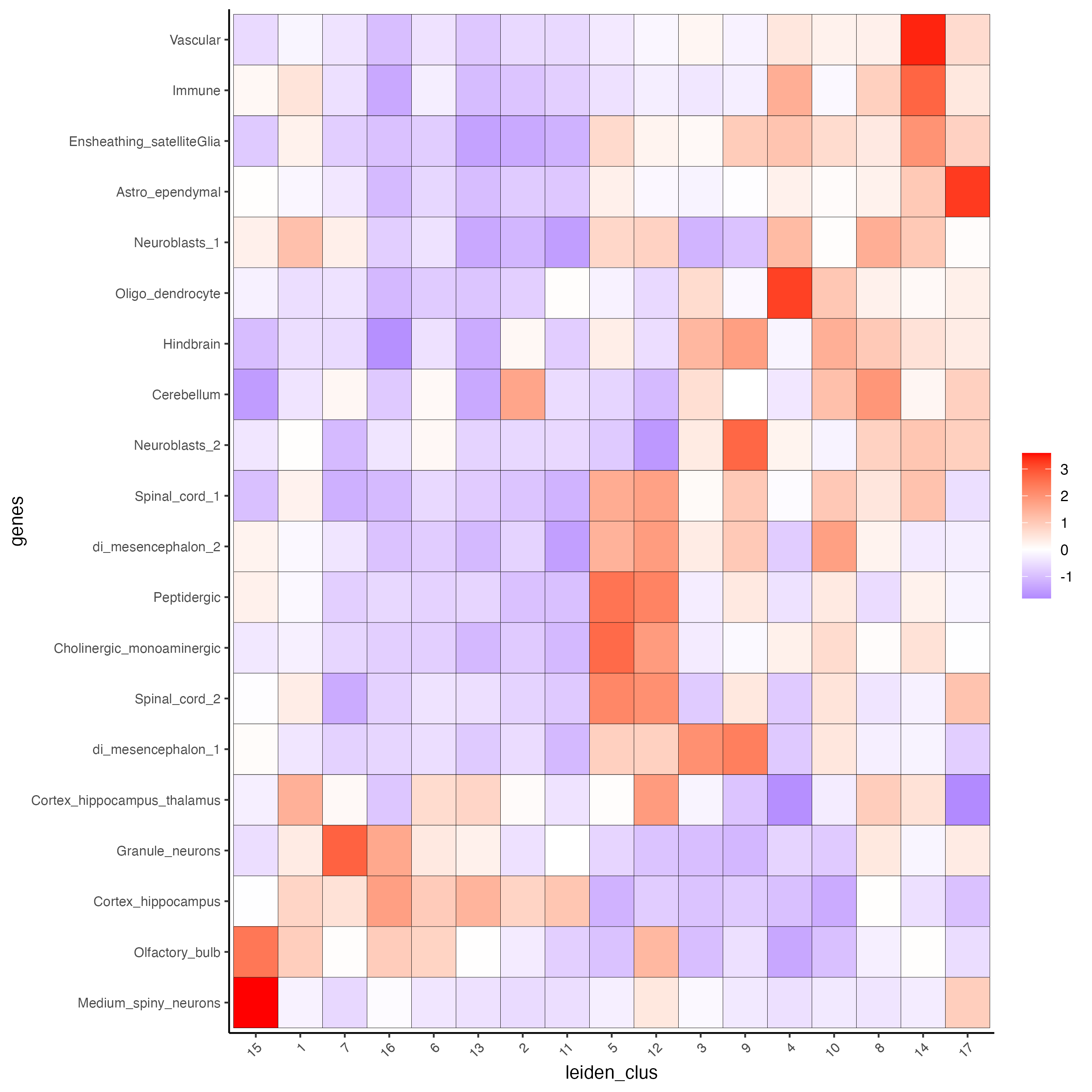
# 1.5 heatmap of enrichment versus annotation (e.g. clustering result)
cell_types_PAGE = colnames(PAGE_matrix_2)
plotMetaDataCellsHeatmap(gobject = visium_brain,
metadata_cols = 'leiden_clus',
value_cols = cell_types_PAGE,
spat_enr_names = 'PAGE',
x_text_size = 8,
y_text_size = 8)
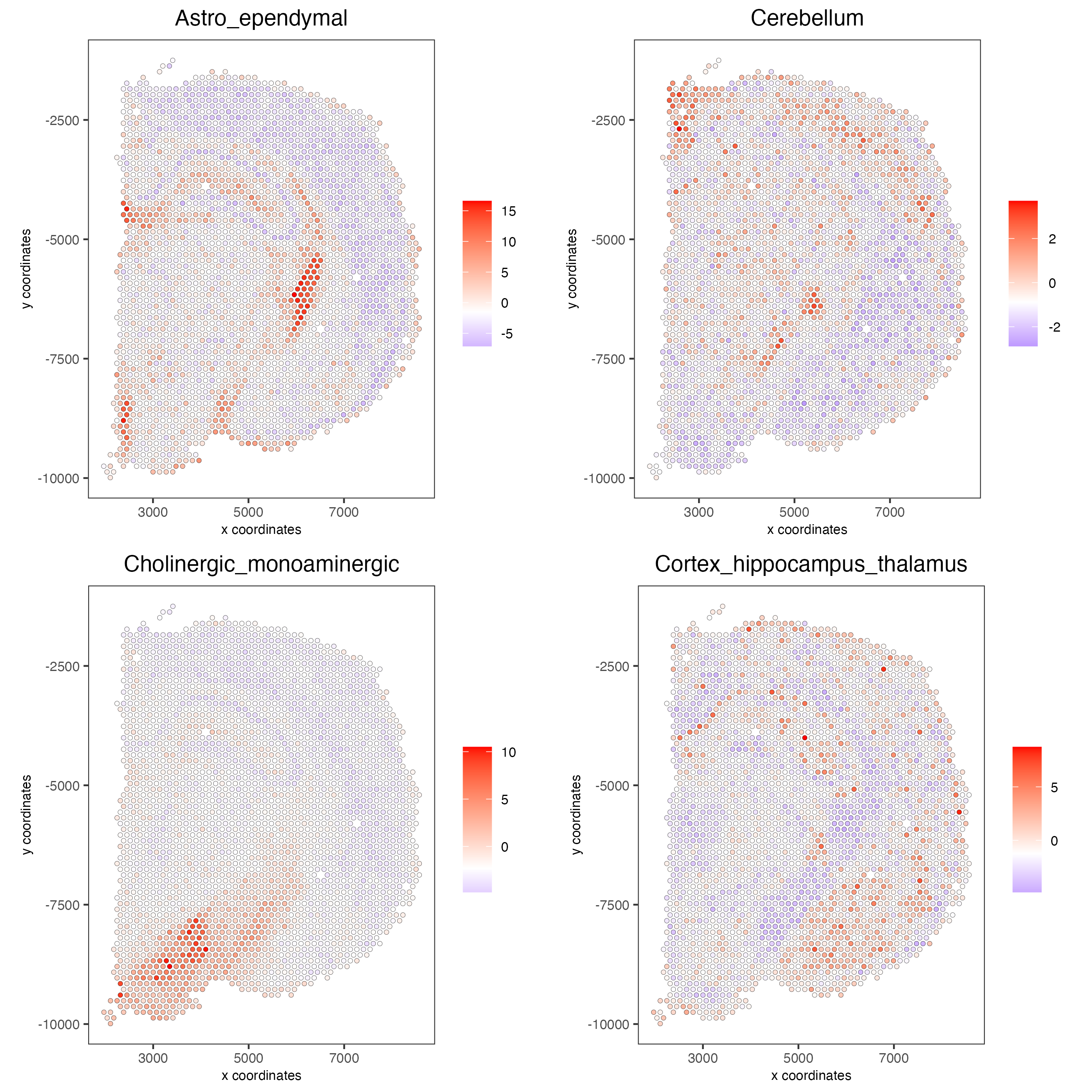
# 1.6 visualizations
spatCellPlot2D(gobject = visium_brain,
               spat_enr_names = 'PAGE',
               cell_annotation_values = cell_types_PAGE[1:4],
               cow_n_col = 2,coord_fix_ratio = 1, point_size = 1.25, show_legend = T)
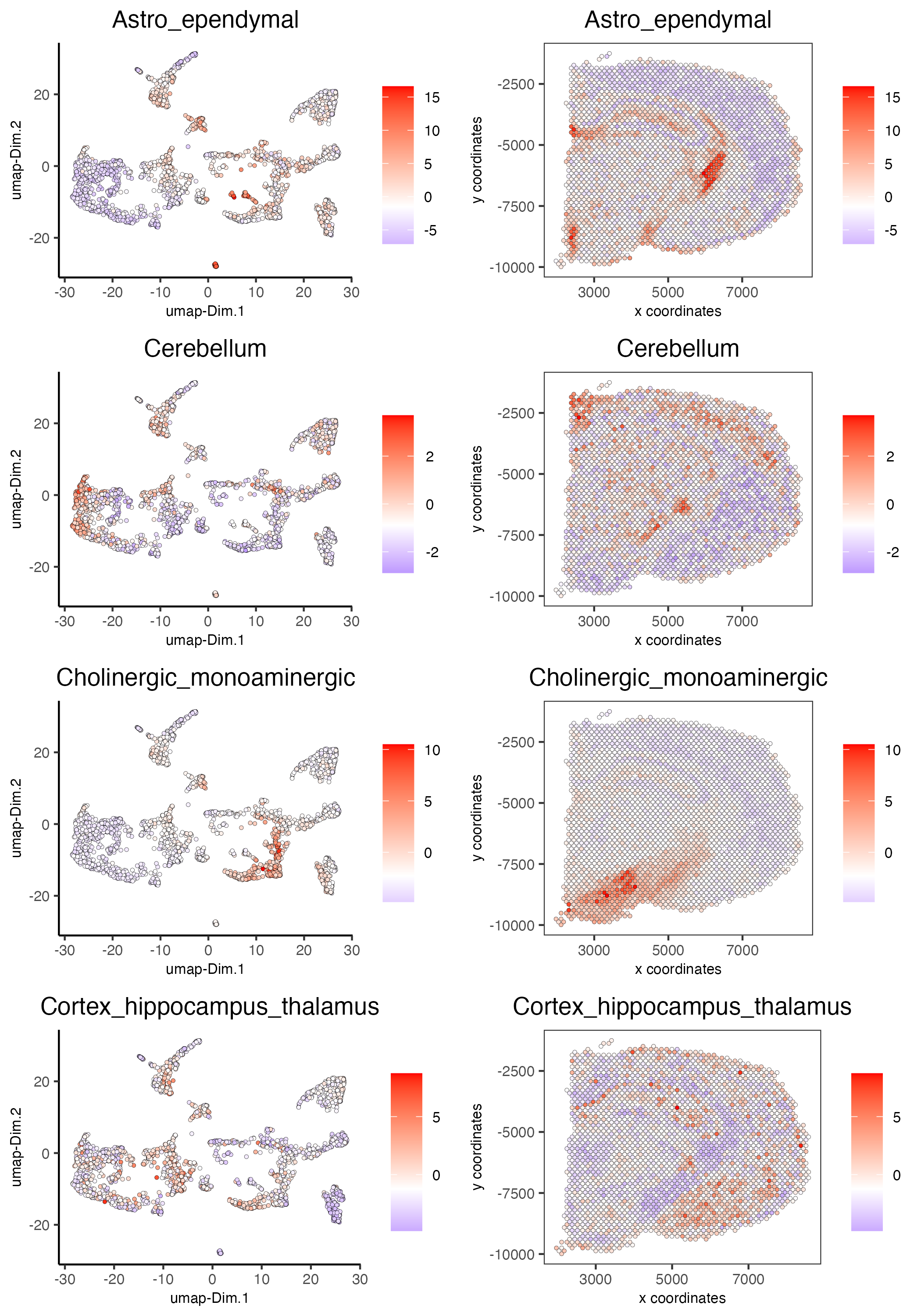
spatDimCellPlot2D(gobject = visium_brain,
                  spat_enr_names = 'PAGE',
                  cell_annotation_values = cell_types_PAGE[1:4],
                  cow_n_col = 1, spat_point_size = 1,
                  plot_alignment = 'horizontal',
                  save_param = list(base_width=7, base_height=10))
7.2 HyperGeometric test#
visium_brain = runHyperGeometricEnrich(gobject = visium_brain,
expression_values = "normalized",
sign_matrix = PAGE_matrix_2)
cell_types_HyperGeometric = colnames(PAGE_matrix_2)
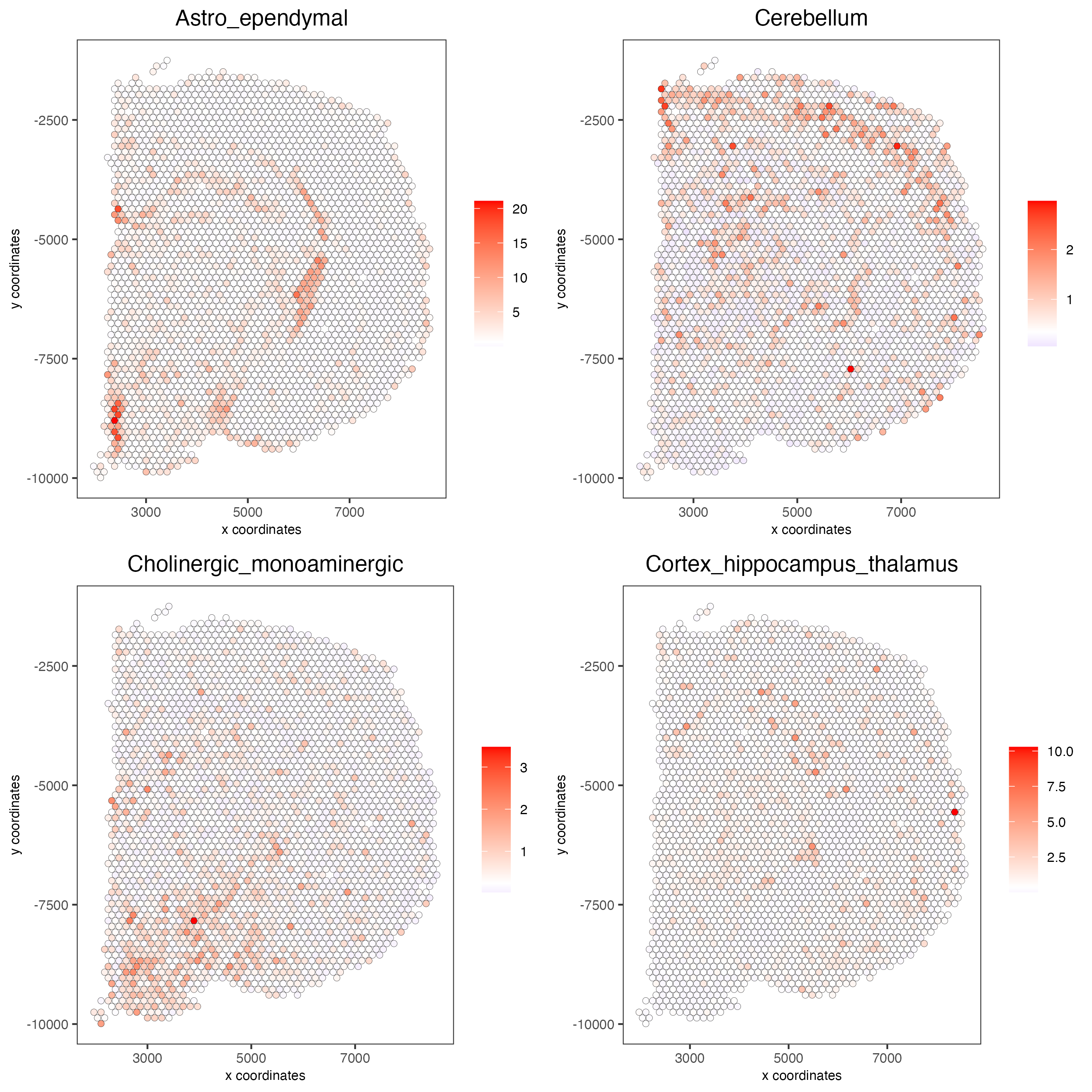
spatCellPlot(gobject = visium_brain,
spat_enr_names = 'hypergeometric',
cell_annotation_values = cell_types_HyperGeometric[1:4],
cow_n_col = 2,coord_fix_ratio = NULL, point_size = 1.75)
7.3 Rank Enrichment#
# Create rank matrix, not that rank matrix is different from PAGE
# A count matrix and a vector for all cell labels will be needed
rank_matrix = makeSignMatrixRank(sc_matrix = get_expression_values(giotto_SC,values = "normalized",output = "matrix"),
                                 sc_cluster_ids = pDataDT(giotto_SC)$Class)
colnames(rank_matrix)<-levels(factor(pDataDT(giotto_SC)$Class))
visium_brain = runRankEnrich(gobject = visium_brain, sign_matrix = rank_matrix,expression_values = "normalized")

# Plot Rank enrichment result
spatCellPlot2D(gobject = visium_brain,
               spat_enr_names = 'rank',
               cell_annotation_values = colnames(rank_matrix)[1:4],
               cow_n_col = 2,coord_fix_ratio = 1, point_size = 1,
               save_param = list(save_name = "spat_enr_Rank_plot"))
7.4 DWLS spatial deconvolution#
# Create DWLS matrix, not that DWLS matrix is different from PAGE and rank
# A count matrix a vector for a list of gene signatures and a vector for all cell labels will be needed
DWLS_matrix<-makeSignMatrixDWLSfromMatrix(matrix = get_expression_values(giotto_SC,values = "normalized",output = "matrix"),
                                          cell_type = pDataDT(giotto_SC)$Class,
                                          sign_gene = top_markers$feats)
visium_brain = runDWLSDeconv(gobject = visium_brain, sign_matrix = DWLS_matrix)


# Plot DWLS deconvolution result
spatCellPlot2D(gobject = visium_brain,
               spat_enr_names = 'DWLS',
               cell_annotation_values = levels(factor(pDataDT(giotto_SC)$Class))[1:4],
               cow_n_col = 2,coord_fix_ratio = 1, point_size = 1,
               save_param = list(save_name = "DWLS_plot"))
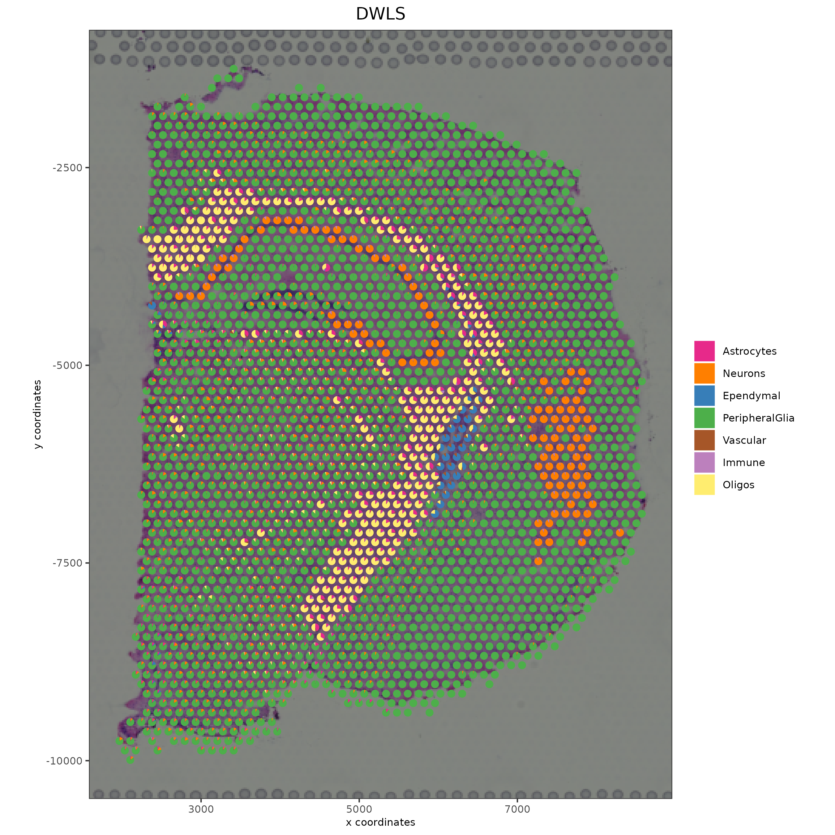
# Plot DWLS deconvolution result with Pie plots
  spatDeconvPlot(visium_brain,
           show_image = T,
           radius = 50,
           save_param = list(save_name = "spat_DWLS_pie_plot"))
Part 8: Spatial Grid#
visium_brain <- createSpatialGrid(gobject = visium_brain,
                                  sdimx_stepsize = 400,
                                  sdimy_stepsize = 400,
                                  minimum_padding = 0)

showGiottoSpatGrids(visium_brain)

spatPlot2D(visium_brain, cell_color = 'leiden_clus', show_grid = T,
           grid_color = 'red', spatial_grid_name = 'spatial_grid')

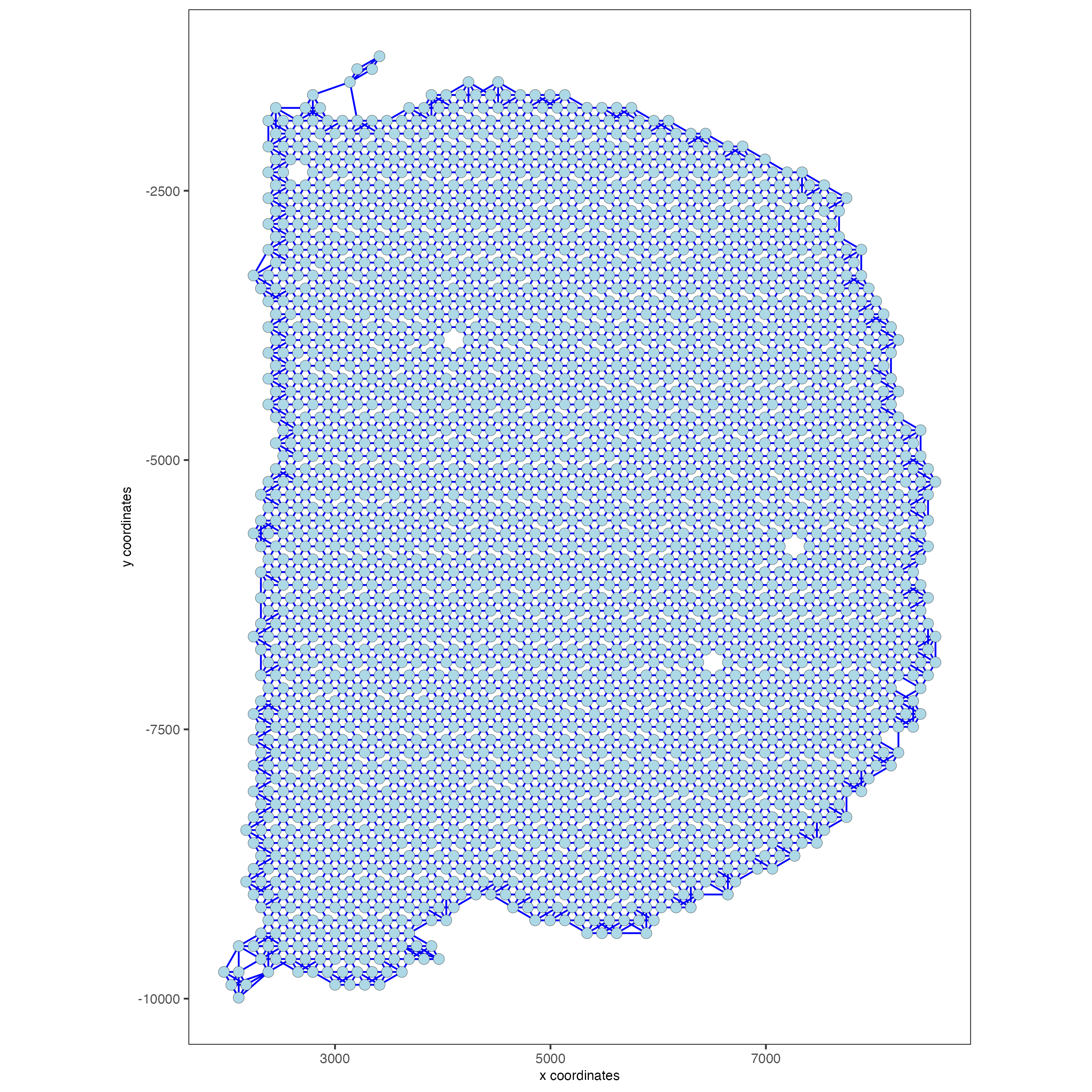
Part 9: spatial network#
visium_brain <- createSpatialNetwork(gobject = visium_brain,
                                     method = 'kNN', k = 5,
                                     maximum_distance_knn = 400,
                                     name = 'spatial_network')

showGiottoSpatNetworks(visium_brain)

spatPlot2D(gobject = visium_brain,  show_network= T,
           network_color = 'blue', spatial_network_name = 'spatial_network')
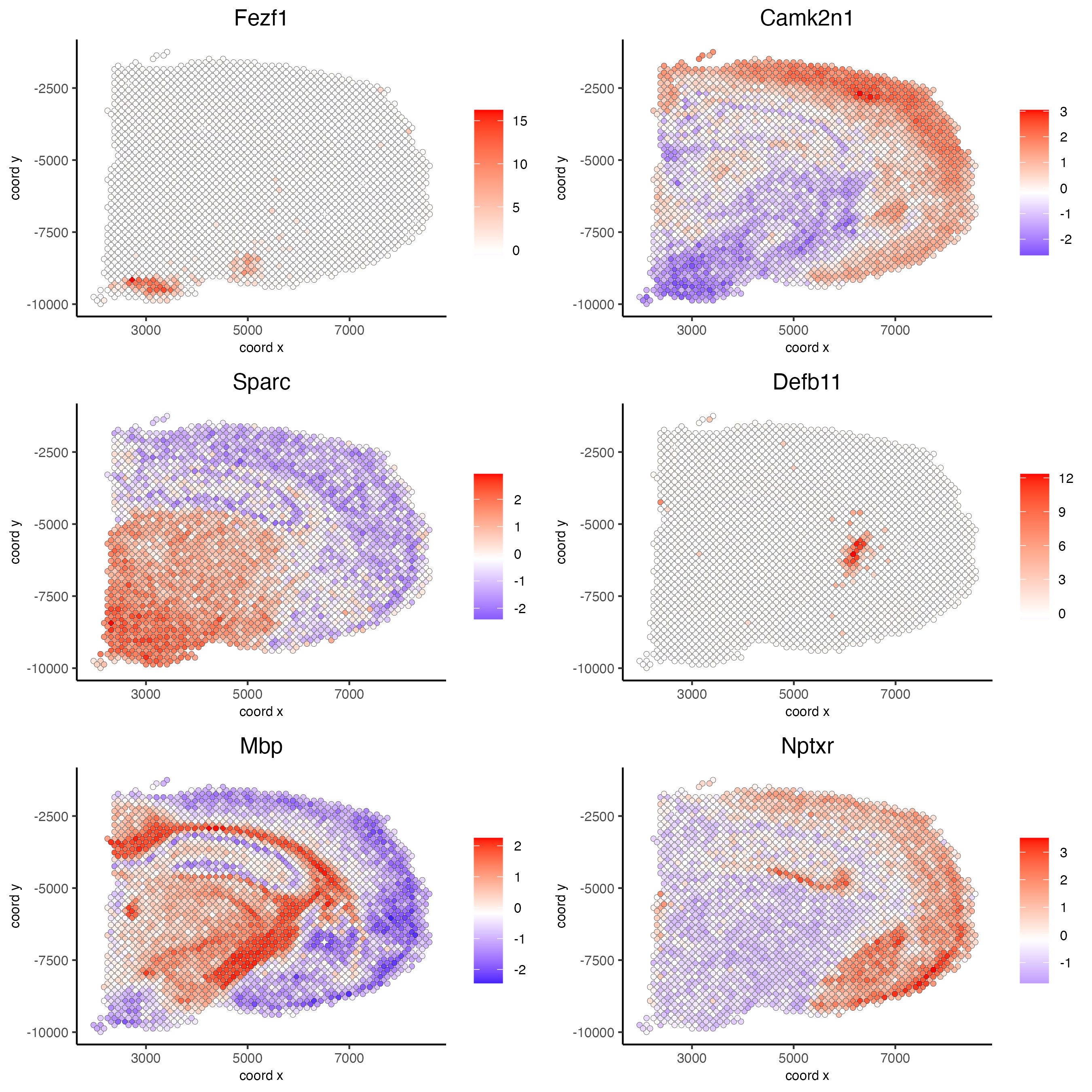
Part 10: Spatial Genes#
## rank binarization
ranktest = binSpect(visium_brain, bin_method = 'rank',
                    calc_hub = T, hub_min_int = 5,
                    spatial_network_name = 'spatial_network')

spatFeatPlot2D(visium_brain, expression_values = 'scaled',
               feats = ranktest$feats[1:6], cow_n_col = 2, point_size = 1.5)
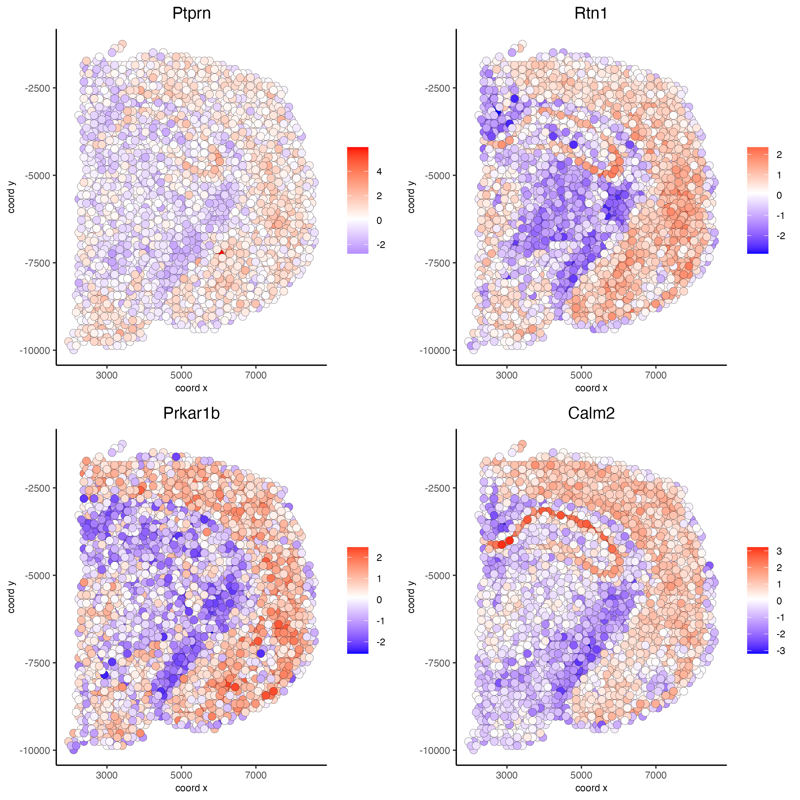
Part 11: Spatial Co-Expression modules#
# cluster the top 500 spatial genes into 20 clusters
ext_spatial_genes = ranktest[1:1500,]$feats

# here we use existing detectSpatialCorGenes function to calculate pairwise distances between genes (but set network_smoothing=0 to use default clustering)
spat_cor_netw_DT = detectSpatialCorFeats(visium_brain,
                                         method = 'network',
                                         spatial_network_name = 'spatial_network',
                                         subset_feats = ext_spatial_genes)

# 2. identify most similar spatially correlated genes for one gene
top10_genes = showSpatialCorFeats(spat_cor_netw_DT, feats = 'Ptprn', show_top_feats = 10)

spatFeatPlot2D(visium_brain, expression_values = 'scaled',
               feats = top10_genes$variable[1:4], point_size = 3)
# cluster spatial genes
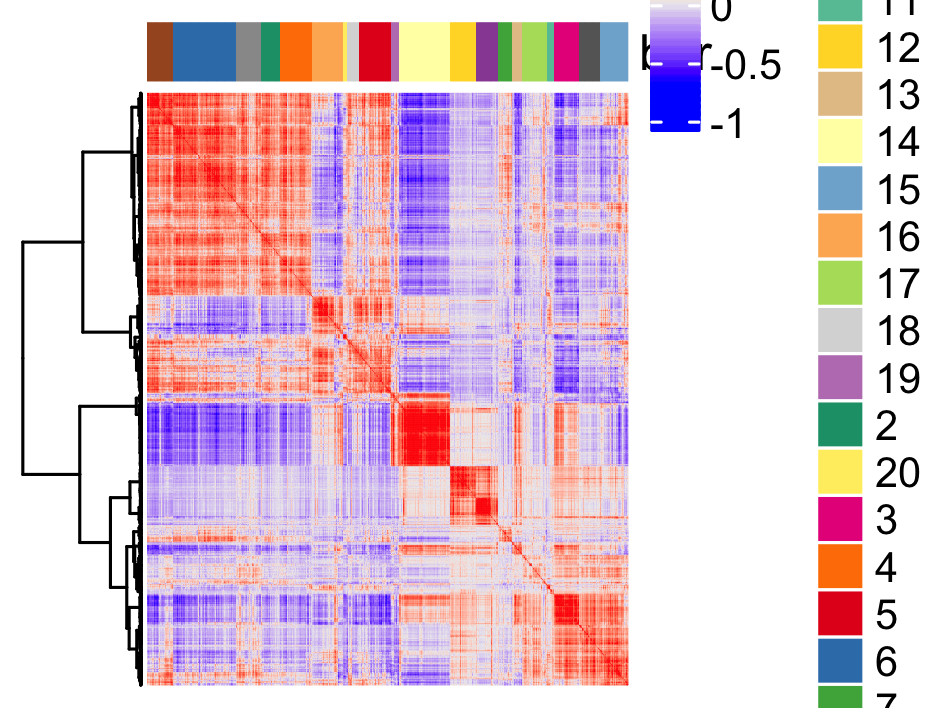
spat_cor_netw_DT = clusterSpatialCorFeats(spat_cor_netw_DT, name = 'spat_netw_clus', k = 20)
# visualize clusters
heatmSpatialCorFeats(visium_brain,
spatCorObject = spat_cor_netw_DT,
use_clus_name = 'spat_netw_clus',
heatmap_legend_param = list(title = NULL),
save_param = list(base_height = 6, base_width = 8, units = 'cm'))
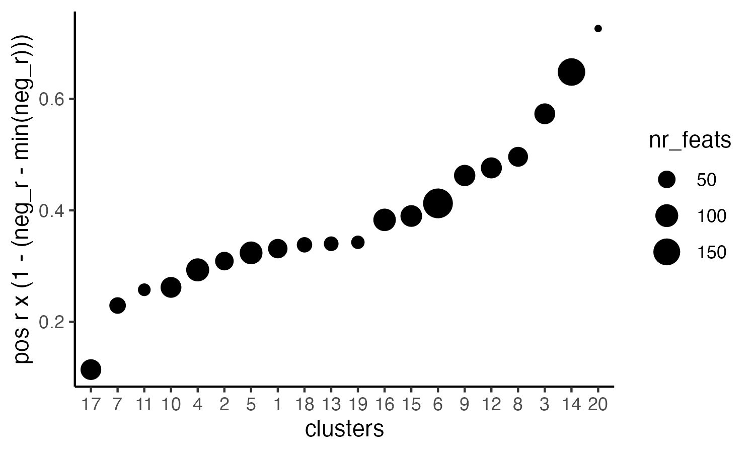
# 4. rank spatial correlated clusters and show genes for selected clusters
netw_ranks = rankSpatialCorGroups(visium_brain,
                                  spatCorObject = spat_cor_netw_DT, use_clus_name = 'spat_netw_clus',
                                  save_param = list(  base_height = 3, base_width = 5))


top_netw_spat_cluster = showSpatialCorFeats(spat_cor_netw_DT, use_clus_name = 'spat_netw_clus',
                                            selected_clusters = 6, show_top_feats = 1)
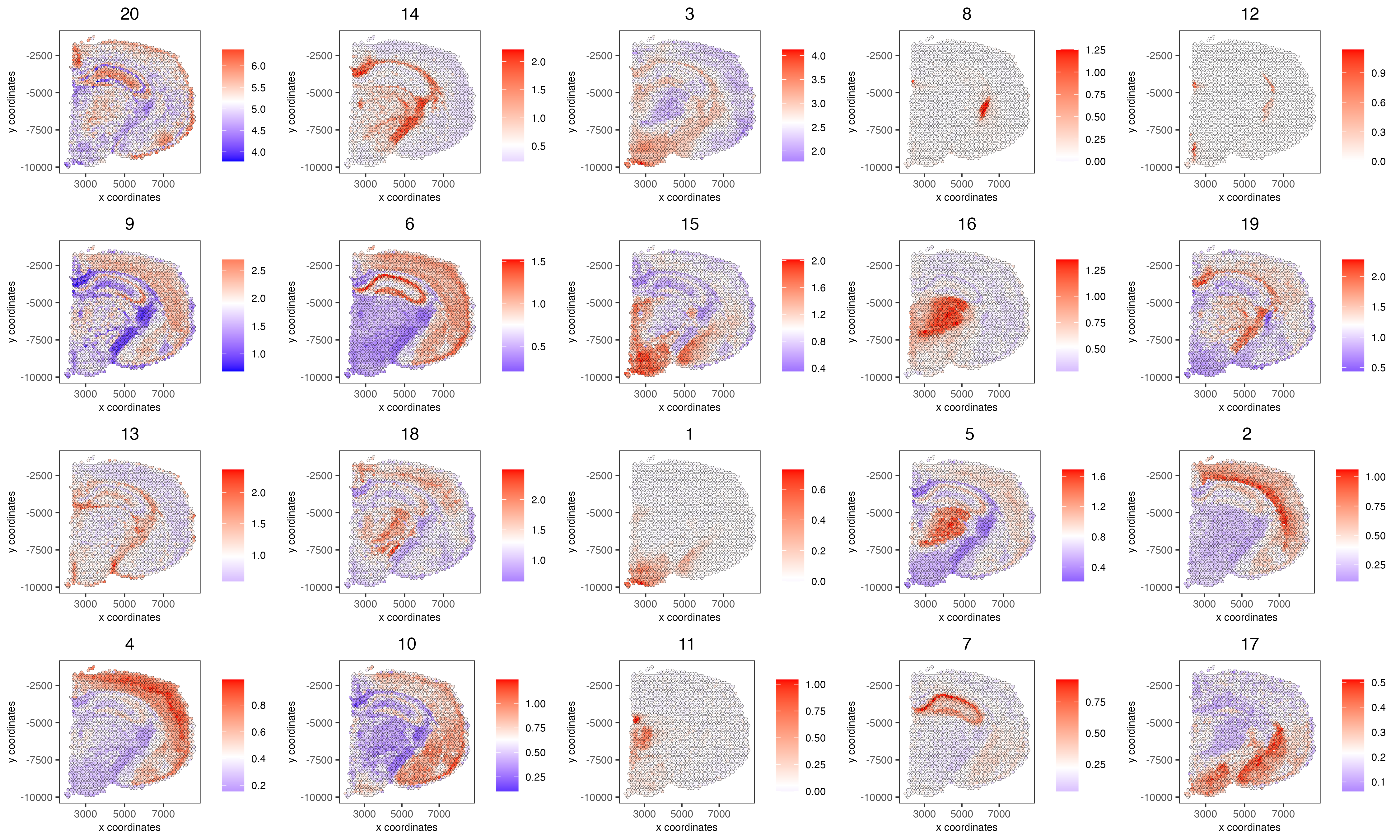
# 5. create metagene enrichment score for clusters
cluster_genes_DT = showSpatialCorFeats(spat_cor_netw_DT, use_clus_name = 'spat_netw_clus', show_top_feats = 1)
cluster_genes = cluster_genes_DT$clus; names(cluster_genes) = cluster_genes_DT$feat_ID

visium_brain = createMetafeats(visium_brain, feat_clusters = cluster_genes, name = 'cluster_metagene')

#showGiottoSpatEnrichments(visium_brain)

spatCellPlot(visium_brain,
             spat_enr_names = 'cluster_metagene',
             cell_annotation_values = netw_ranks$clusters,
             point_size = 1, cow_n_col = 5, save_param = list(base_width = 15))
Part 12: Spatially informed clusters#
# top 30 genes per spatial co-expression cluster
table(spat_cor_netw_DT$cor_clusters$spat_netw_clus)
coexpr_dt = data.table::data.table(genes = names(spat_cor_netw_DT$cor_clusters$spat_netw_clus),
cluster = spat_cor_netw_DT$cor_clusters$spat_netw_clus)
data.table::setorder(coexpr_dt, cluster)
top30_coexpr_dt = coexpr_dt[, head(.SD, 30) , by = cluster]
my_spatial_genes <- top30_coexpr_dt$genes
visium_brain <- runPCA(gobject = visium_brain,
feats_to_use = my_spatial_genes,
name = 'custom_pca')
visium_brain <- runUMAP(visium_brain, dim_reduction_name = 'custom_pca', dimensions_to_use = 1:20,
name = 'custom_umap')
visium_brain <- createNearestNetwork(gobject = visium_brain,
dim_reduction_name = 'custom_pca',
dimensions_to_use = 1:20, k = 5,
name = 'custom_NN')
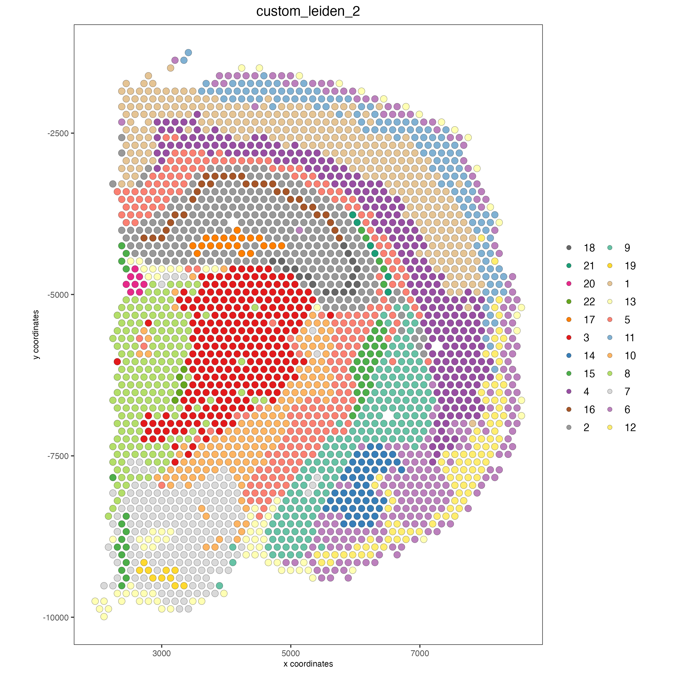
visium_brain <- doLeidenCluster(gobject = visium_brain, network_name = 'custom_NN',
resolution = 0.15, n_iterations = 1000,
name = 'custom_leiden')
cell_meta = pDataDT(visium_brain)
cell_clusters = unique(cell_meta$custom_leiden)
selected_colors = getDistinctColors(length(cell_clusters))
names(selected_colors) = cell_clusters
spatPlot2D(visium_brain, cell_color = 'custom_leiden', cell_color_code = selected_colors, coord_fix_ratio = 1)
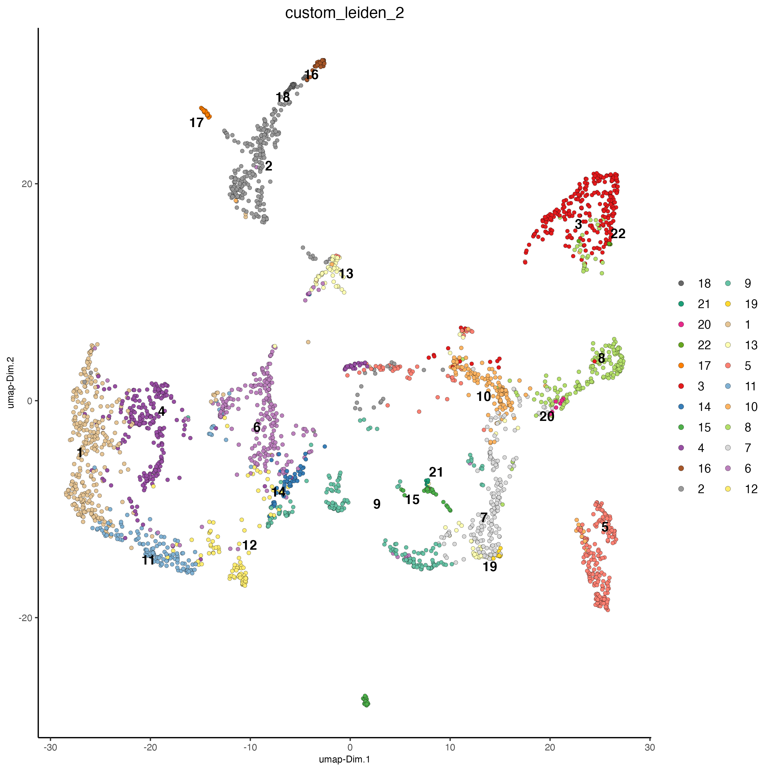
plotUMAP(gobject = visium_brain, cell_color = 'custom_leiden', cell_color_code = selected_colors, point_size = 1.5)
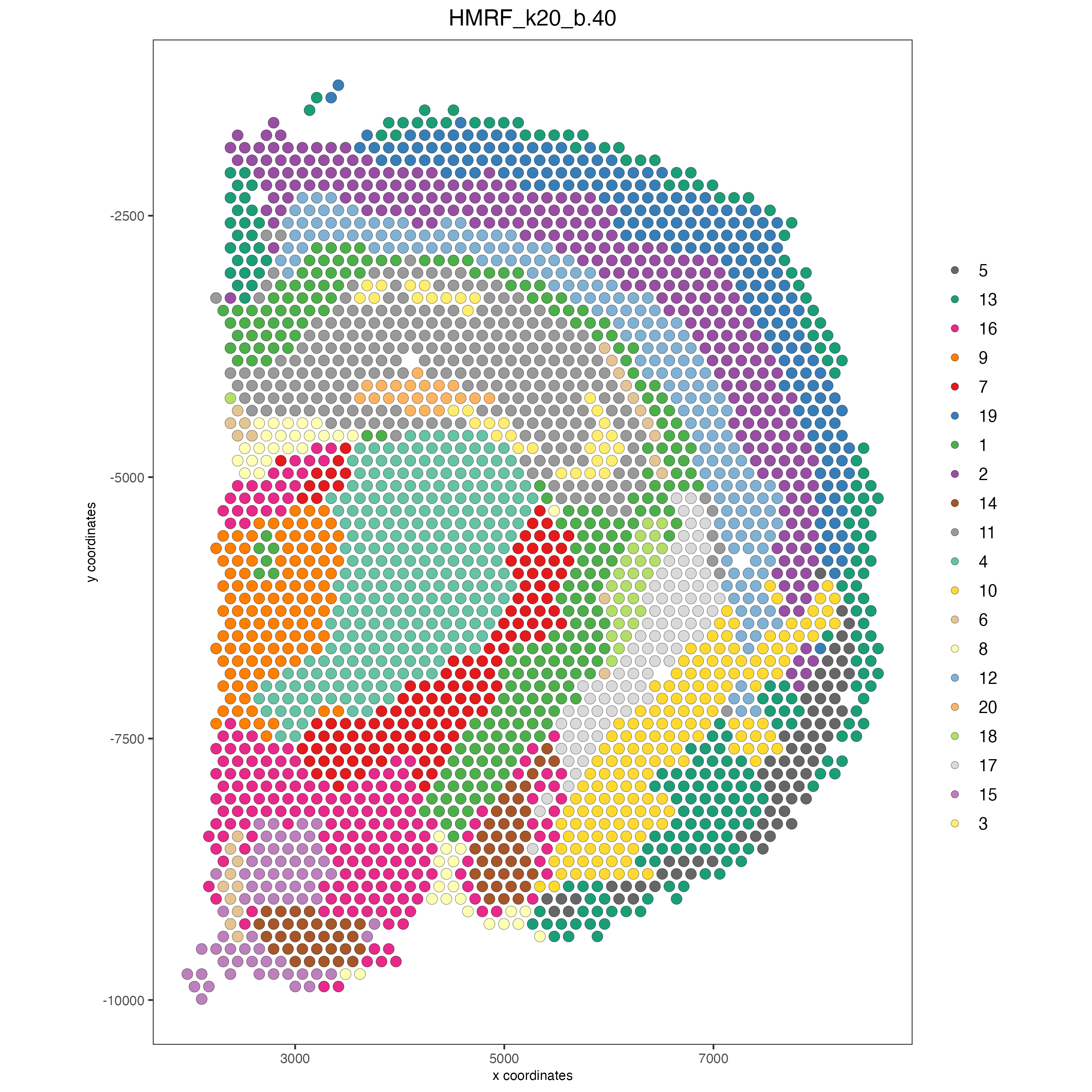
Part 13: Spatial domains with HMRF#
# do HMRF with different betas on top 30 genes per spatial co-expression module
hmrf_folder = paste0(results_folder,'/','11_HMRF/')
if(!file.exists(hmrf_folder)) dir.create(hmrf_folder, recursive = T)

HMRF_spatial_genes = doHMRF(gobject = visium_brain,
                            expression_values = 'scaled',
                            spatial_genes = my_spatial_genes, k = 20,
                            spatial_network_name="spatial_network",
                            betas = c(0, 10, 5),
                            output_folder = paste0(hmrf_folder, '/', 'Spatial_genes/SG_topgenes_k20_scaled'))

visium_brain = addHMRF(gobject = visium_brain, HMRFoutput = HMRF_spatial_genes,
                       k = 20, betas_to_add = c(0, 10, 20, 30, 40),
                       hmrf_name = 'HMRF')

spatPlot2D(gobject = visium_brain, cell_color = 'HMRF_k20_b.40')