Visium Prostate Integration#
- Date:
5/5/23
1 Start Giotto#
# Ensure Giotto Suite is installed
if(!"Giotto" %in% installed.packages()) {
  devtools::install_github("drieslab/Giotto@suite")
}
library(Giotto)

# Ensure Giotto Data is installed
if(!"GiottoData" %in% installed.packages()) {
  devtools::install_github("drieslab/GiottoData")
}
library(GiottoData)

# Ensure the Python environment for Giotto has been installed
genv_exists = checkGiottoEnvironment()
if(!genv_exists){
  # The following command need only be run once to install the Giotto environment
  installGiottoEnvironment()
}
# 1. set working directory
results_directory = getwd()

# 2. set giotto python path
# set python path to your preferred python version path
# set python path to NULL if you want to automatically install (only the 1st time) and use the giotto miniconda environment
python_path = NULL
if(is.null(python_path)) {
  installGiottoEnvironment()
}
 giotto environment found at
my/path/r-miniconda\envs\giotto_env\python.exe
Giotto environment is already installed, set force_environment = TRUE to
 reinstall
# 3. create giotto instructions
instrs = createGiottoInstructions(save_dir = results_directory,
                                  save_plot = TRUE,
                                  show_plot = TRUE,
                                  python_path = python_path)
no external python path was provided, but a giotto python environment was found
 and will be used
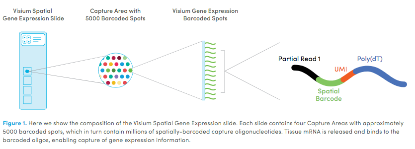
2 Dataset explanation#
10X genomics recently launched a new platform to obtain spatial expression data using a Visium Spatial Gene Expression slide.
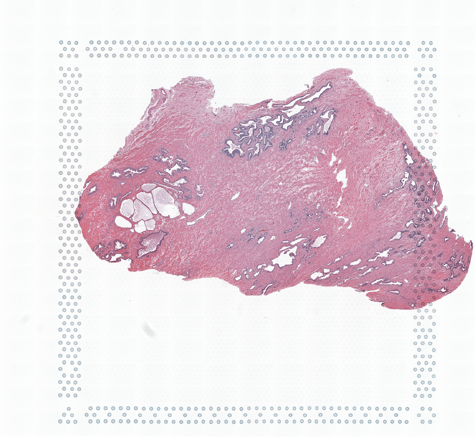
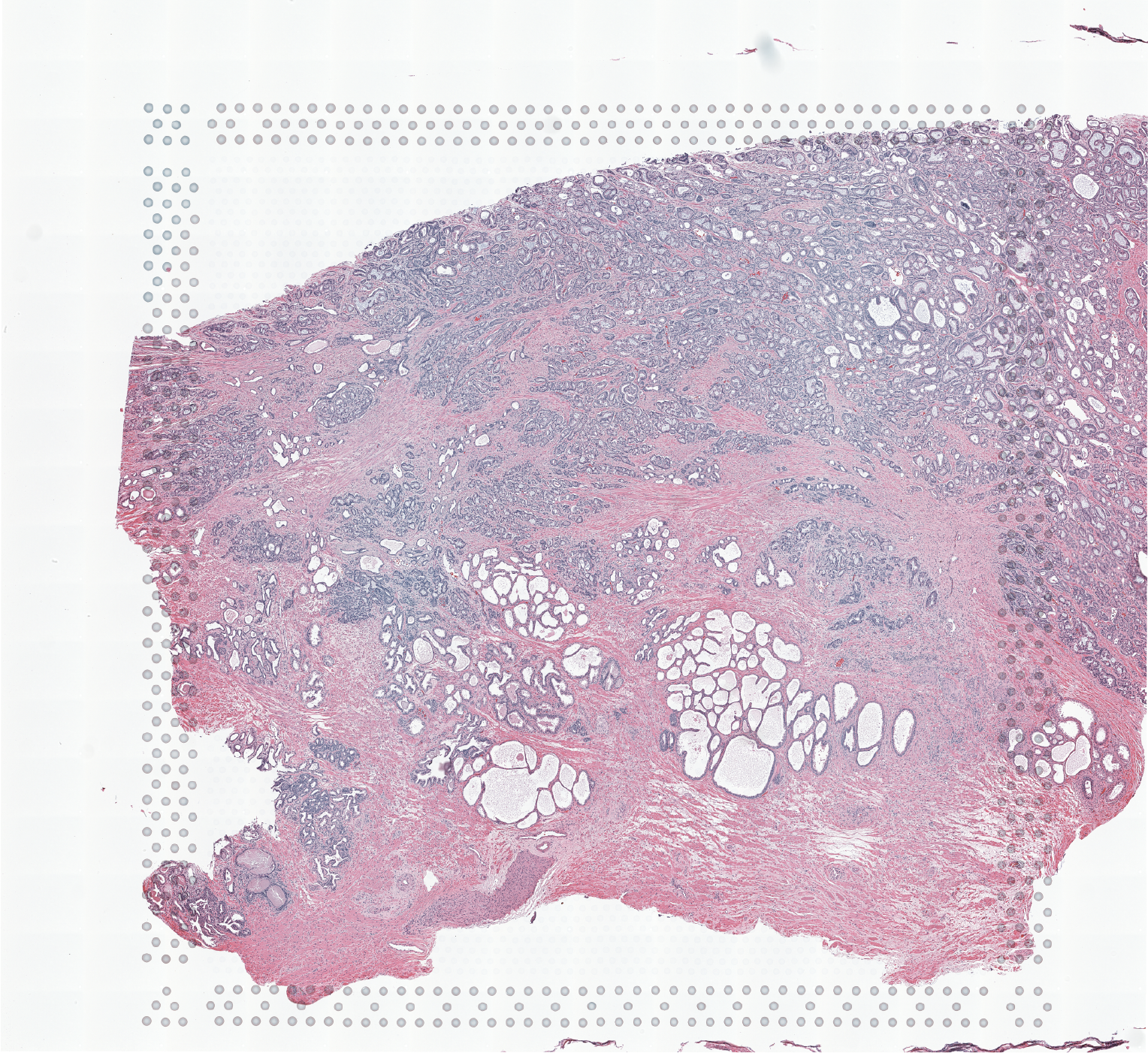
The Visium Cancer Prostate data to run this tutorial can be found here The Visium Normal Prostate data to run this tutorial can be found here
3 Create Giotto objects and join#
# This dataset must be downlaoded manually; please do so and change the path below as appropriate
data_directory <- getwd()

## obese upper
N_pros = createGiottoVisiumObject(
    visium_dir = paste0(data_directory,'/Visium_FFPE_Human_Normal_Prostate'),
    expr_data = 'raw',
    png_name = 'tissue_lowres_image.png',
    gene_column_index = 2,
    instructions = instrs
)
A structured visium directory will be used
png and scalefactors paths are found and automatic alignment for the lowres
 image will be attempted
Consider to install these (optional) packages to run all possible Giotto
 commands for spatial analyses: MAST tiff biomaRt trendsceek multinet RTriangle
 FactoMineR
Giotto does not automatically install all these packages as they are not
 absolutely required and this reduces the number of dependencies
## obese lower
C_pros = createGiottoVisiumObject(
    visium_dir = paste0(data_directory,'/Visium_FFPE_Human_Prostate_Cancer/'),
    expr_data = 'raw',
    png_name = 'tissue_lowres_image.png',
    gene_column_index = 2,
    instructions = instrs
)
A structured visium directory will be used
png and scalefactors paths are found and automatic alignment for the lowres
 image will be attempted
Consider to install these (optional) packages to run all possible Giotto
 commands for spatial analyses: MAST tiff biomaRt trendsceek multinet RTriangle
 FactoMineR
Giotto does not automatically install all these packages as they are not
 absolutely required and this reduces the number of dependencies
# join giotto objects
# joining with x_shift has the advantage that you can join both 2D and 3D data
# x_padding determines how much distance is between each dataset
# if x_shift = NULL, then the total shift will be guessed from the giotto image
testcombo = joinGiottoObjects(gobject_list = list(N_pros, C_pros),
    gobject_names = c('NP', 'CP'),
    join_method = 'shift', x_padding = 1000)
> raw already exists and will be replaced with new spatial locations
> raw already exists and will be replaced with new spatial locations
# join info is stored in this slot
# simple list for now
testcombo@join_info
$list_IDs
[1] "NP" "CP"

$join_method
[1] "shift"

$z_vals
[1] 1000

$x_shift
NULL

$y_shift
NULL

$x_padding
[1] 1000

$y_padding
[1] 0
# check joined Giotto object
fDataDT(testcombo)
                          feat_ID
    1:                      OR4F5
    2:                     SAMD11
    3:                      NOC2L
    4:                     KLHL17
    5:                    PLEKHN1
   ---
18753: DEPRECATED_ENSG00000164220
18754: DEPRECATED_ENSG00000178287
18755: DEPRECATED_ENSG00000198203
18756: DEPRECATED_ENSG00000284667
18757: DEPRECATED_ENSG00000284704
pDataDT(testcombo)
                    cell_ID in_tissue array_row array_col list_ID
   1: NP-AAACAACGAATAGTTC-1         0         0        16      NP
   2: NP-AAACAAGTATCTCCCA-1         1        50       102      NP
   3: NP-AAACAATCTACTAGCA-1         1         3        43      NP
   4: NP-AAACACCAATAACTGC-1         0        59        19      NP
   5: NP-AAACAGAGCGACTCCT-1         1        14        94      NP
  ---
9979: CP-TTGTTTCACATCCAGG-1         1        58        42      CP
9980: CP-TTGTTTCATTAGTCTA-1         1        60        30      CP
9981: CP-TTGTTTCCATACAACT-1         1        45        27      CP
9982: CP-TTGTTTGTATTACACG-1         0        73        41      CP
9983: CP-TTGTTTGTGTAAATTC-1         1         7        51      CP
showGiottoImageNames(testcombo)
Image type: image

--> Name: NP-image
--> Name: CP-image
showGiottoSpatLocs(testcombo)
└──Spatial unit "cell"
   └──S4 spatLocsObj "raw" coordinates:   (9983 rows)
         An object of class spatLocsObj
         provenance: cell
             ------------------------
            sdimx  sdimy               cell_ID
         1:  7419  -3686 NP-AAACAACGAATAGTTC-1
         2: 19873 -16327 NP-AAACAAGTATCTCCCA-1
         3: 11334  -4450 NP-AAACAATCTACTAGCA-1
         4:  7829 -18579 NP-AAACACCAATAACTGC-1

         ranges:
              sdimx  sdimy
         [1,]  5066 -23288
         [2,] 52011  -3682
showGiottoExpression(testcombo)
└──Spatial unit "cell"
   └──Feature type "rna"
      └──Expression data "raw" values:
            An object of class exprObj
            for spatial unit: "cell" and feature type: "rna"
              Provenance:  cell

            contains:
            18757 x 9983 sparse Matrix of class "dgCMatrix"

            A1BG . . . .  . . . . . . . . ......
            A1CF . . . .  . . . . . . . . ......
            A2M  2 8 . . 15 4 2 . . . 2 3 ......

             ........suppressing 9971 columns and 18751 rows

            ZYG11B . 1 . . . . . . . . . . ......
            ZYX    . 1 1 . 5 2 . . . . . 1 ......
            ZZEF1  . 1 . . 3 . . . . . . . ......

             First four colnames:
             NP-AAACAACGAATAGTTC-1
             NP-AAACAAGTATCTCCCA-1
             NP-AAACAATCTACTAGCA-1
             NP-AAACACCAATAACTGC-1
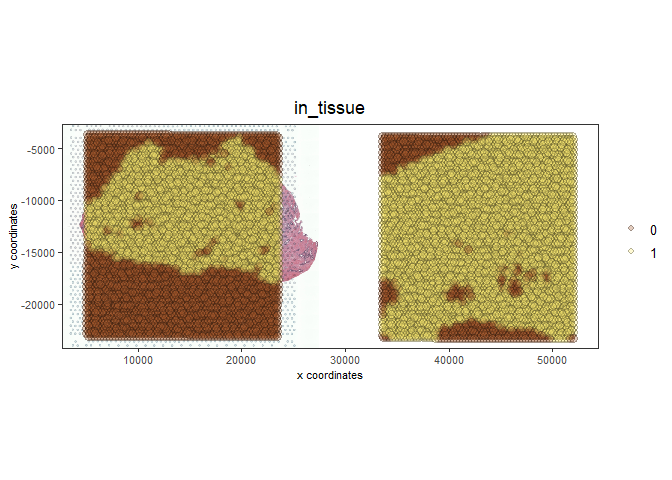
# this plots all the images by list_ID
spatPlot2D(gobject = testcombo, cell_color = 'in_tissue',
    show_image = T, image_name = c("NP-image", "CP-image"),
    group_by = 'list_ID', point_alpha = 0.5,
    save_param = list(save_name = "1a_plot"))
# this plots one selected image
spatPlot2D(gobject = testcombo, cell_color = 'in_tissue',
    show_image = T, image_name = c("NP-image"), point_alpha = 0.3,
    save_param = list(save_name = "1b_plot"))
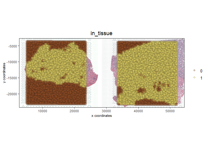
# this plots two selected images
spatPlot2D(gobject = testcombo, cell_color = 'in_tissue',
    show_image = T, image_name = c( "NP-image", "CP-image"),
    point_alpha = 0.3,
    save_param = list(save_name = "1c_plot"))
4 Process Giotto Objects#
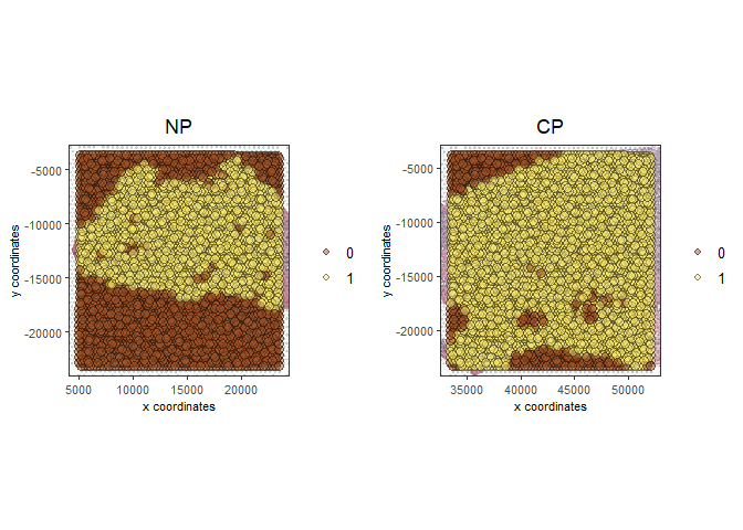
# subset on in-tissue spots
metadata = pDataDT(testcombo)
in_tissue_barcodes = metadata[in_tissue == 1]$cell_ID
testcombo = subsetGiotto(testcombo, cell_ids = in_tissue_barcodes)
## filter
testcombo <- filterGiotto(gobject = testcombo,
    expression_threshold = 1,
    feat_det_in_min_cells = 50,
    min_det_feats_per_cell = 500,
    expression_values = c('raw'),
    verbose = T)
completed 1: preparation
completed 2: subset expression data
completed 3: subset spatial locations
completed 4: subset cell (spatial units) and feature IDs
completed 5: subset cell metadata
completed 6: subset feature metadata
completed 7: subset spatial network(s)
completed 8: subsetted dimension reductions
completed 9: subsetted nearest network(s)
completed 10: subsetted spatial enrichment results
number of frames:  25
sys parent:  24
NULL
$cell
$cell$raw
An object of class spatLocsObj
for spatial unit: "cell"
provenance: cell
   ------------------------

preview:
      sdimx  sdimy               cell_ID
   1: 19873 -16327 NP-AAACAAGTATCTCCCA-1
   2: 11334  -4450 NP-AAACAATCTACTAGCA-1
   3: 18728  -7239 NP-AAACAGAGCGACTCCT-1
   4:  6385 -14538 NP-AAACAGCTTTCAGAAG-1
   5: 21761 -15069 NP-AAACCCGAACGAAATC-1
  ---
6907: 44746 -11665 CP-TTGTTGTGTGTCAAGA-1
6908: 39658 -18473 CP-TTGTTTCACATCCAGG-1
6909: 37916 -18975 CP-TTGTTTCATTAGTCTA-1
6910: 37487 -15188 CP-TTGTTTCCATACAACT-1
6911: 40983  -5601 CP-TTGTTTGTGTAAATTC-1

ranges:
     sdimx  sdimy
[1,]  5081 -23287
[2,] 52011  -3839


Feature type:  rna
Number of cells removed:  3  out of  6914
Number of feats removed:  3591  out of  18757
## normalize
testcombo <- normalizeGiotto(gobject = testcombo, scalefactor = 6000)
first scale feats and then cells
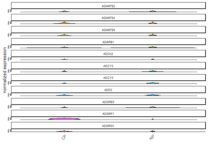
## add gene & cell statistics
testcombo <- addStatistics(gobject = testcombo, expression_values = 'raw')

fmeta = fDataDT(testcombo)
testfeats = fmeta[perc_cells > 20 & perc_cells < 50][100:110]$feat_ID

violinPlot(testcombo, feats = testfeats, cluster_column = 'list_ID', save_param = list(save_name = "2a_plot"))
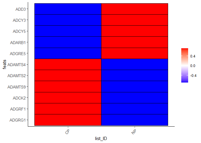
plotMetaDataHeatmap(testcombo, selected_feats = testfeats, metadata_cols = 'list_ID', save_param = list(save_name = "2b_plot"))
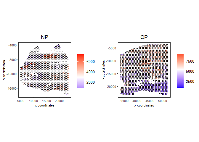
## visualize
spatPlot2D(gobject = testcombo, group_by = 'list_ID', cell_color = 'nr_feats', color_as_factor = F, point_size = 0.75, save_param = list(save_name = "2c_plot"))
5 Dimention Reduction#
## PCA ##
testcombo <- calculateHVF(gobject = testcombo)
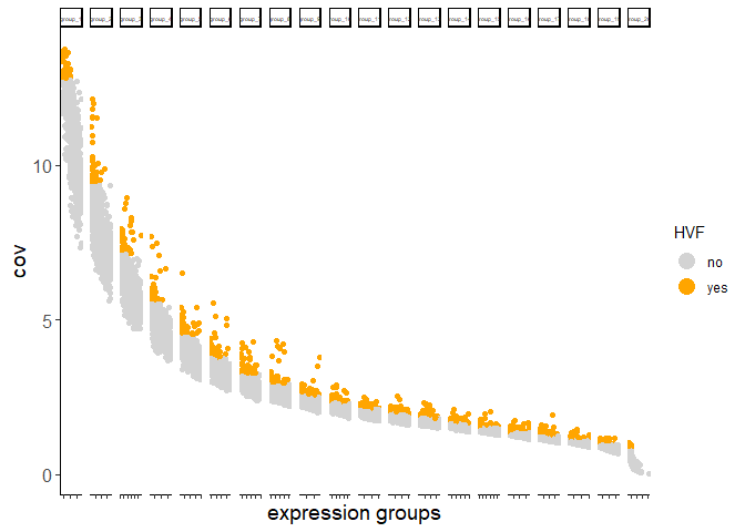
return_plot = TRUE and return_gobject = TRUE

          plot will not be returned to object, but can still be saved with save_plot = TRUE or manually
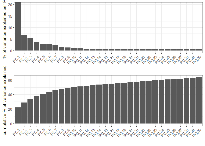
testcombo <- runPCA(gobject = testcombo, center = TRUE, scale_unit = TRUE)
"hvf" was found in the feats metadata information and will be used to select
 highly variable features
class of selected matrix: dgCMatrix
screePlot(testcombo, ncp = 30, save_param = list(save_name = "3a_screeplot"))
PCA with name: pca already exists and will be used for the screeplot
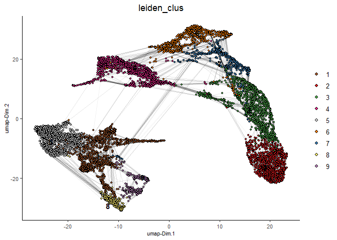
6 Clustering#
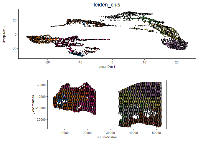
6.1 Without Integration#
Integration is usually needed for dataset of different conditions to minimize batch effects. Without integration means without using any integration methods.
## cluster and run UMAP ##
# sNN network (default)
testcombo <- createNearestNetwork(gobject = testcombo,
    dim_reduction_to_use = 'pca', dim_reduction_name = 'pca',
    dimensions_to_use = 1:10, k = 15)

# Leiden clustering
testcombo <- doLeidenCluster(gobject = testcombo, resolution = 0.2, n_iterations = 1000)

# UMAP
testcombo = runUMAP(testcombo)

plotUMAP(gobject = testcombo,
    cell_color = 'leiden_clus', show_NN_network = T, point_size = 1.5,
    save_param = list(save_name = "4.1a_plot"))
spatPlot2D(gobject = testcombo, group_by = 'list_ID',
    cell_color = 'leiden_clus',
    point_size = 1.5,
    save_param = list(save_name = "4.1b_plot"))
spatDimPlot2D(gobject = testcombo,
    cell_color = 'leiden_clus',
    save_param = list(save_name = "4.1c_plot"))
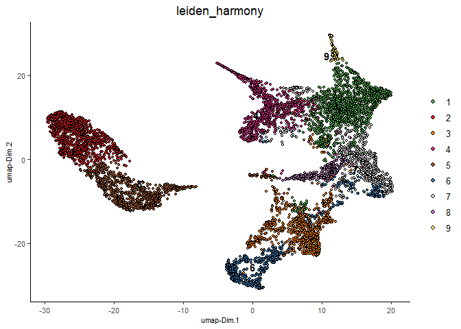
6.2 With Harmony integration#
Harmony is a integration algorithm developed by Korsunsky, I. et al.. It was designed for integration of single cell data but also work well on spatial datasets.
## data integration, cluster and run UMAP ##

# harmony
#library(devtools)
#install_github("immunogenomics/harmony")
library(harmony)
Loading required package: Rcpp
Warning: package 'Rcpp' was built under R version 4.2.3
## run harmony integration
testcombo = runGiottoHarmony(testcombo, vars_use = 'list_ID', do_pca = F)
using 'Harmony' to integrate different datasets. If used in published research, please cite:

  Korsunsky, I., Millard, N., Fan, J. et al.
                      Fast, sensitive and accurate integration of single-cell data with Harmony.
                      Nat Methods 16, 1289-1296 (2019).
                      https://doi.org/10.1038/s41592-019-0619-0
Harmony 1/10
Harmony 2/10
Harmony 3/10
Harmony 4/10
Harmony converged after 4 iterations
## sNN network (default)
testcombo <- createNearestNetwork(gobject = testcombo,
    dim_reduction_to_use = 'harmony', dim_reduction_name = 'harmony', name = 'NN.harmony',
    dimensions_to_use = 1:10, k = 15)

## Leiden clustering
testcombo <- doLeidenCluster(gobject = testcombo,
    network_name = 'NN.harmony', resolution = 0.2, n_iterations = 1000, name = 'leiden_harmony')

# UMAP dimension reduction
testcombo = runUMAP(testcombo, dim_reduction_name = 'harmony', dim_reduction_to_use = 'harmony', name = 'umap_harmony')


plotUMAP(gobject = testcombo,
    dim_reduction_name = 'umap_harmony',
    cell_color = 'leiden_harmony',
    show_NN_network = F,
    point_size = 1.5,
    save_param = list(save_name = "4.2a_plot"))
# If you want to show NN network information, you will need to specify these arguments in the plotUMAP function
# show_NN_network = T, nn_network_to_use = 'sNN' , network_name = 'NN.harmony'
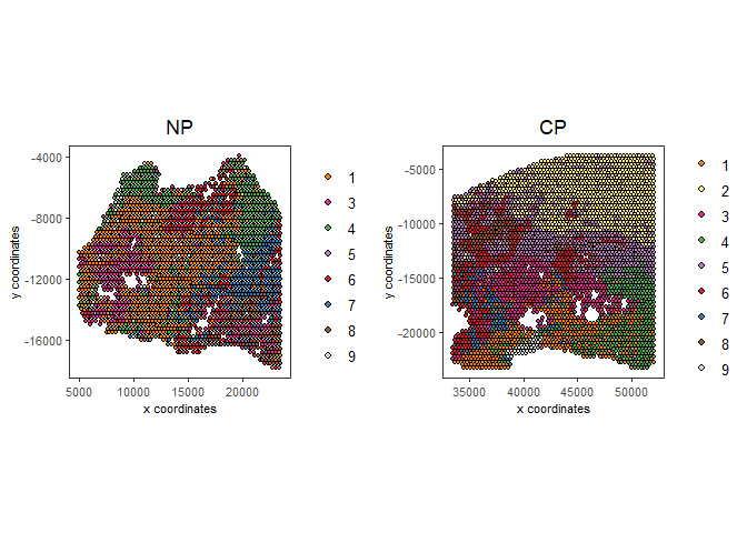
spatPlot2D(gobject = testcombo, group_by = 'list_ID',
    cell_color = 'leiden_harmony',
    point_size = 1.5,
    save_param = list(save_name = "4.2b_plot"))
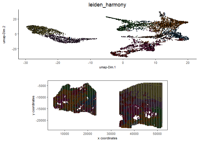
spatDimPlot2D(gobject = testcombo,
    dim_reduction_to_use = 'umap', dim_reduction_name = 'umap_harmony',
    cell_color = 'leiden_harmony',
    save_param = list(save_name = "4.2c_plot"))
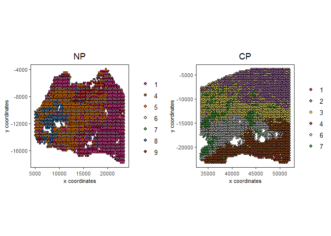
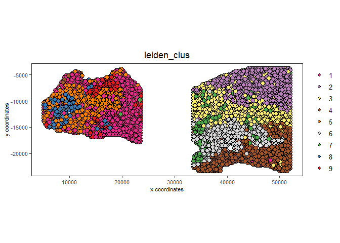
# compare to previous results
spatPlot2D(gobject = testcombo,
    cell_color = 'leiden_clus',
    save_param = list(save_name = "4_w_o_integration_plot"))
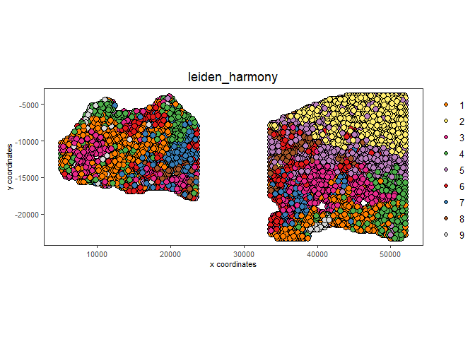
spatPlot2D(gobject = testcombo,
    cell_color = 'leiden_harmony',
    save_param = list(save_name = "4_w_integration_plot"))
7 Cell type annotation#
This is also the easiest way to integrate Visium datasets with single cell data. Example shown here is from Ma et al. from two prostate cancer patients. The raw dataset can be found here Giotto_SC is processed variable in the single cell RNAseq tutorial. You can also get access to the processed files of this dataset using getSpatialDataset
# download data to results directory ####
# if wget is installed, set method = 'wget'
# if you run into authentication issues with wget, then add " extra = '--no-check-certificate' "
getSpatialDataset(dataset = 'scRNA_prostate', directory = data_directory)
Selected dataset links for: scRNA_prostate
          dataset spatial_locs
1: scRNA_prostate
                                                                                                                                   expr_matrix
1: https://github.com/drieslab/spatial-datasets/raw/master/data/2022_scRNAseq_human_prostate/count_matrix/prostate_sc_expression_matrix.csv.gz
                                                                                                                           metadata
1: https://github.com/drieslab/spatial-datasets/raw/master/data/2022_scRNAseq_human_prostate/cell_metadata/prostate_sc_metadata.csv
Download expression matrix:
Download spatial locations:
No spatial locations found, skip this step
Download metadata:
sc_expression = paste0(data_directory, "/prostate_sc_expression_matrix.csv.gz")
sc_metadata = paste0(data_directory, "/prostate_sc_metadata.csv")

giotto_SC <- createGiottoObject(
  expression = sc_expression,
  instructions = instrs
)
Consider to install these (optional) packages to run all possible Giotto
 commands for spatial analyses: MAST tiff biomaRt trendsceek multinet RTriangle
 FactoMineR
Giotto does not automatically install all these packages as they are not
 absolutely required and this reduces the number of dependencies
There are non numeric or integer columns for the spatial location input at
 column position(s): 1
 The first non-numeric column will be considered as a cell ID to test for
 consistency with the expression matrix
 Other non numeric columns will be removed
giotto_SC <- addCellMetadata(giotto_SC,
                             new_metadata = data.table::fread(sc_metadata))

giotto_SC<- normalizeGiotto(giotto_SC)
first scale feats and then cells
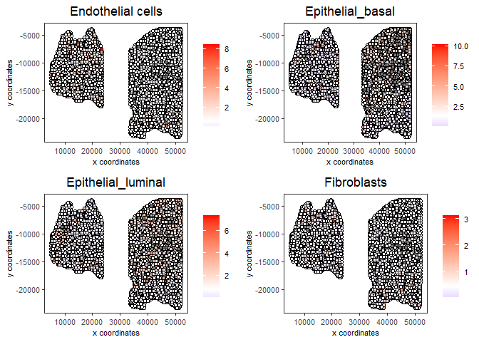
7.1 PAGE enrichment#
# Create PAGE matrix
# PAGE matrix should be a binary matrix with each row represent a gene marker and each column represent a cell type
# markers_scran is generated from single cell analysis ()
markers_scran = findMarkers_one_vs_all(gobject=giotto_SC,
                                       method="scran",
                                       expression_values="normalized",
                                       cluster_column='prostate_labels',
                                       min_feats=3)
using 'Scran' to detect marker feats. If used in published research, please cite:
  Lun ATL, McCarthy DJ, Marioni JC (2016).
  'A step-by-step workflow for low-level analysis of single-cell RNA-seq data with Bioconductor.'
  F1000Res., 5, 2122. doi: 10.12688/f1000research.9501.2.
start with cluster  Endothelial cells

start with cluster  Epithelial_basal

start with cluster  Epithelial_luminal

start with cluster  Fibroblasts

start with cluster  Macrophage & B cells

start with cluster  Mast cells

start with cluster  Mesenchymal cells

start with cluster  Neural Progenitor cells

start with cluster  Smooth muscle cells

start with cluster  T cells
top_markers <- markers_scran[, head(.SD, 10), by="cluster"]
celltypes<-levels(factor(markers_scran$cluster))
sign_list<-list()

for (i in 1:length(celltypes)){
  sign_list[[i]]<-top_markers[which(top_markers$cluster == celltypes[i]),]$feats
}

PAGE_matrix = makeSignMatrixPAGE(sign_names = celltypes,
                                 sign_list = sign_list)
testcombo = runPAGEEnrich(gobject = testcombo,
sign_matrix = PAGE_matrix,
min_overlap_genes = 2)
cell_types_subset = colnames(PAGE_matrix)
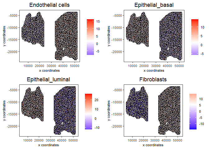
# Plot PAGE enrichment result
spatCellPlot(gobject = testcombo,
spat_enr_names = 'PAGE',
cell_annotation_values = cell_types_subset[1:4],
cow_n_col = 2,coord_fix_ratio = NULL, point_size = 1.25,
save_param = list(save_name = "5a_PAGE_plot"))
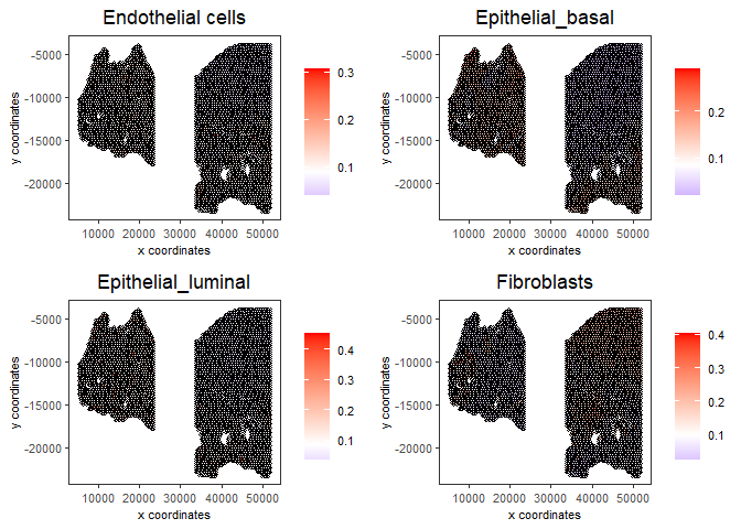
7.2 Hypergeometric test#
testcombo = runHyperGeometricEnrich(gobject = testcombo,
                                    expression_values = "normalized",
                                    sign_matrix = PAGE_matrix)
cell_types_subset = colnames(PAGE_matrix)
spatCellPlot(gobject = testcombo,
             spat_enr_names = 'hypergeometric',
             cell_annotation_values = cell_types_subset[1:4],
             cow_n_col = 2,coord_fix_ratio = NULL, point_size = 1.75,
             save_param = list(save_name = "5b_HyperGeometric_plot"))
7.3 Rank Enrichment#
# Create rank matrix, not that rank matrix is different from PAGE
# A count matrix and a vector for all cell labels will be needed
sc_expression_norm = getExpression(giotto_SC,
                                  values = "normalized",
                                  output = "matrix")

prostate_feats = pDataDT(giotto_SC)$prostate_label

rank_matrix = makeSignMatrixRank(sc_matrix = sc_expression_norm,
                                 sc_cluster_ids = prostate_feats)
colnames(rank_matrix)<-levels(factor(prostate_feats))
testcombo = runRankEnrich(gobject = testcombo, sign_matrix = rank_matrix,expression_values = "normalized")

# Plot Rank enrichment result
spatCellPlot2D(gobject = testcombo,
               spat_enr_names = 'rank',
               cell_annotation_values = cell_types_subset[1:4],
               cow_n_col = 2,coord_fix_ratio = NULL, point_size = 1,
               save_param = list(save_name = "5c_Rank_plot"))
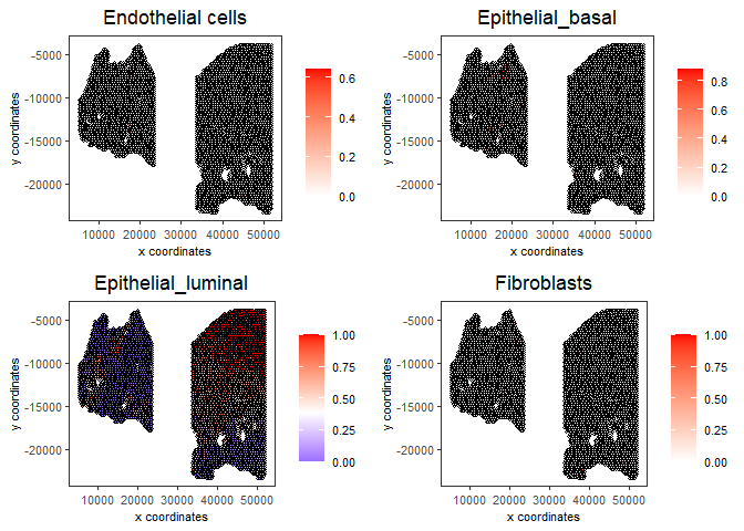
7.4 DWLS Deconvolution#
# Create DWLS matrix, not that DWLS matrix is different from PAGE and rank
# A count matrix a vector for a list of gene signatures and a vector for all cell labels will be needed
DWLS_matrix<-makeSignMatrixDWLSfromMatrix(matrix = sc_expression_norm,
                                          cell_type = prostate_feats,
                                          sign_gene = top_markers$feats)
testcombo = runDWLSDeconv(gobject = testcombo, sign_matrix = DWLS_matrix)


# Plot DWLS deconvolution result
spatCellPlot2D(gobject = testcombo,
               spat_enr_names = 'DWLS',
               cell_annotation_values = levels(factor(prostate_feats))[1:4],
               cow_n_col = 2,coord_fix_ratio = NULL, point_size = 1,
               save_param = list(save_name = "5d_DWLS_plot"))
8 Session Info#
sessionInfo()
R version 4.2.2 (2022-10-31 ucrt)
Platform: x86_64-w64-mingw32/x64 (64-bit)
Running under: Windows 10 x64 (build 22621)

Matrix products: default

locale:
[1] LC_COLLATE=English_United States.utf8
[2] LC_CTYPE=English_United States.utf8
[3] LC_MONETARY=English_United States.utf8
[4] LC_NUMERIC=C
[5] LC_TIME=English_United States.utf8

attached base packages:
[1] stats     graphics  grDevices utils     datasets  methods   base

other attached packages:
[1] harmony_0.1.1    Rcpp_1.0.10      GiottoData_0.2.1 Giotto_3.3.0
[5] testthat_3.1.5

loaded via a namespace (and not attached):
  [1] systemfonts_1.0.4           plyr_1.8.8
  [3] igraph_1.4.1                lazyeval_0.2.2
  [5] sp_1.6-0                    BiocParallel_1.32.6
  [7] listenv_0.9.0               usethis_2.1.6
  [9] GenomeInfoDb_1.34.6         ggplot2_3.4.2
 [11] digest_0.6.30               htmltools_0.5.4
 [13] magick_2.7.4                fansi_1.0.4
 [15] magrittr_2.0.3              memoise_2.0.1
 [17] ScaledMatrix_1.6.0          cluster_2.1.4
 [19] limma_3.54.2                remotes_2.4.2
 [21] globals_0.16.2              matrixStats_0.63.0
 [23] R.utils_2.12.2              prettyunits_1.1.1
 [25] colorspace_2.1-0            rappdirs_0.3.3
 [27] ggrepel_0.9.2               textshaping_0.3.6
 [29] xfun_0.38                   dplyr_1.1.1
 [31] callr_3.7.3                 crayon_1.5.2
 [33] RCurl_1.98-1.9              jsonlite_1.8.3
 [35] progressr_0.13.0            glue_1.6.2
 [37] gtable_0.3.3                zlibbioc_1.44.0
 [39] XVector_0.38.0              DelayedArray_0.24.0
 [41] pkgbuild_1.4.0              BiocSingular_1.14.0
 [43] RcppZiggurat_0.1.6          future.apply_1.10.0
 [45] SingleCellExperiment_1.20.0 BiocGenerics_0.44.0
 [47] scales_1.2.1                edgeR_3.40.1
 [49] miniUI_0.1.1.1              viridisLite_0.4.2
 [51] xtable_1.8-4                dqrng_0.3.0
 [53] reticulate_1.26             rsvd_1.0.5
 [55] stats4_4.2.2                profvis_0.3.7
 [57] metapod_1.6.0               htmlwidgets_1.6.2
 [59] httr_1.4.5                  RColorBrewer_1.1-3
 [61] ellipsis_0.3.2              scuttle_1.8.3
 [63] urlchecker_1.0.1            pkgconfig_2.0.3
 [65] R.methodsS3_1.8.2           farver_2.1.1
 [67] uwot_0.1.14                 deldir_1.0-6
 [69] locfit_1.5-9.7              utf8_1.2.3
 [71] here_1.0.1                  tidyselect_1.2.0
 [73] labeling_0.4.2              rlang_1.1.0
 [75] reshape2_1.4.4              later_1.3.0
 [77] munsell_0.5.0               tools_4.2.2
 [79] cachem_1.0.6                cli_3.4.1
 [81] dbscan_1.1-11               generics_0.1.3
 [83] devtools_2.4.5              evaluate_0.20
 [85] stringr_1.5.0               fastmap_1.1.0
 [87] yaml_2.3.7                  ragg_1.2.4
 [89] processx_3.8.0              knitr_1.42
 [91] fs_1.5.2                    purrr_1.0.1
 [93] future_1.32.0               sparseMatrixStats_1.10.0
 [95] mime_0.12                   scran_1.26.1
 [97] R.oo_1.25.0                 brio_1.1.3
 [99] compiler_4.2.2              rstudioapi_0.14
[101] plotly_4.10.1               png_0.1-7
[103] statmod_1.4.37              tibble_3.2.1
[105] stringi_1.7.8               ps_1.7.2
[107] desc_1.4.2                  bluster_1.8.0
[109] lattice_0.20-45             Matrix_1.5-1
[111] vctrs_0.6.1                 pillar_1.9.0
[113] lifecycle_1.0.3             BiocNeighbors_1.16.0
[115] RcppAnnoy_0.0.20            data.table_1.14.6
[117] cowplot_1.1.1               bitops_1.0-7
[119] irlba_2.3.5.1               httpuv_1.6.6
[121] GenomicRanges_1.50.2        R6_2.5.1
[123] promises_1.2.0.1            IRanges_2.32.0
[125] parallelly_1.35.0           sessioninfo_1.2.2
[127] codetools_0.2-18            pkgload_1.3.2
[129] SummarizedExperiment_1.28.0 rprojroot_2.0.3
[131] withr_2.5.0                 S4Vectors_0.36.2
[133] GenomeInfoDbData_1.2.9      parallel_4.2.2
[135] terra_1.7-18                quadprog_1.5-8
[137] grid_4.2.2                  beachmat_2.14.0
[139] tidyr_1.3.0                 Rfast_2.0.6
[141] DelayedMatrixStats_1.20.0   rmarkdown_2.21
[143] MatrixGenerics_1.10.0       Rtsne_0.16
[145] Biobase_2.58.0              shiny_1.7.4