Spatial Transformations#
- Date:
7/28/23
1 Spatial Object Manipulation#
2 Start Giotto#
# Ensure Giotto Suite is installed
i_p = installed.packages()
if(!"Giotto" %in% i_p) devtools::install_github("drieslab/Giotto@suite")
library(Giotto)

# Ensure Giotto Data is installed
if(!"GiottoData" %in% i_p) devtools::install_github("drieslab/GiottoData")
library(GiottoData)

# Ensure the Python environment for Giotto has been installed
genv_exists = checkGiottoEnvironment()
if(!genv_exists){
  # The following command need only be run once to install the Giotto environment
  installGiottoEnvironment()
}
3 Load mini giotto object example#
First we will load in the a mini dataset put together from Vizgen’s Mouse Brain Receptor Map data release. This mini giotto object has been pre-analyzed and comes with many analyses and data objects attached. Most of these analyses have been performed on the ‘aggregate’ `spatial unit <>`__ so we will set it as the active spatial unit in order to default to it.
viz <- GiottoData::loadGiottoMini(dataset = 'vizgen')
activeSpatUnit(viz) <- 'aggregate'
4 Extract spatial info#
Then we will extract the spatial subobjects that we will use. These will be all subobjects in Giotto that contain coordinates data or directly map their data to space.
image <- getGiottoImage(viz, image_type = 'largeImage', name = 'dapi_z0')
spat_locs <- getSpatialLocations(viz)
spat_net <- getSpatialNetwork(viz)
gpoints <- getFeatureInfo(viz, return_giottoPoints = TRUE)
gpoly <- getPolygonInfo(viz, polygon_name = 'aggregate', return_giottoPolygon = TRUE)
5 Defining bounds and extent#
One of the most convenient descriptors of where an object is in space is
its minima and maxima in the coordinate plane, also known as the
boundaries or spatial extent of that information. It can be thought
of as bounding box around where your information exists in space.
Giotto incorporates usage of the SpatExtent class and associated
ext() generic from terra to describe objects spatially.
ext(image) # giottoLargeImage
SpatExtent : 6400.029, 6900.037, -5150.007, -4699.967 (xmin, xmax, ymin, ymax)
ext(spat_locs) # spatLocsObj
SpatExtent : 6401.41164725267, 6899.10802819571, -5146.74746408943, -4700.32590047134 (xmin, xmax, ymin, ymax)
ext(spat_net) # spatNetObj
SpatExtent : 6401.411647, 6899.108028, -5146.747464, -4700.3259 (xmin, xmax, ymin, ymax)
ext(gpoints) # giottoPoints
SpatExtent : 6400.037, 6900.0317, -5149.9834, -4699.9785 (xmin, xmax, ymin, ymax)
ext(gpoly) # giottoPolygon
SpatExtent : 6391.46568586489, 6903.57332779812, -5153.89721175534, -4694.86823300896 (xmin, xmax, ymin, ymax)
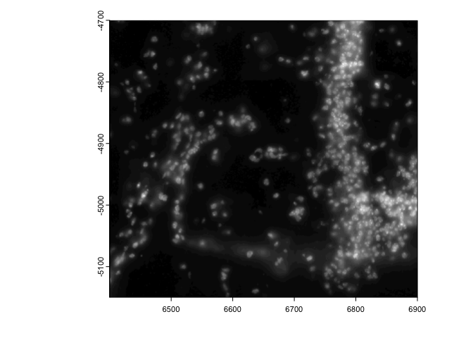
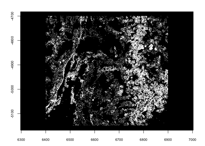
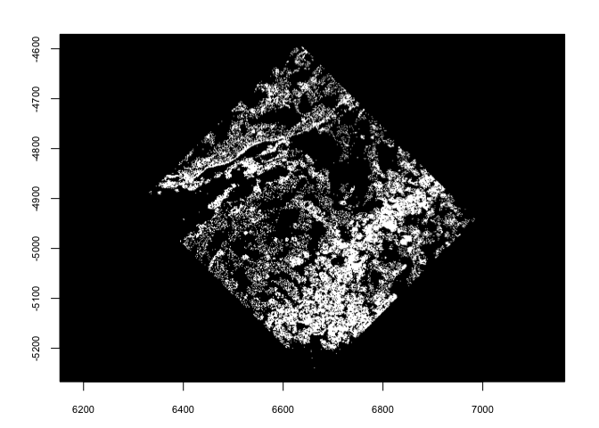
5.1 Image extent#
With giottoLargeImage objects, you are additionally able to assign
how they map to space using ext(). Note that modifications performed
on one giottoLargeImage are applied to all references to that object
unless copy() is used first.
e <- ext(image) # save extent
plot(image)
# modify extent
ext(image) <- c(0,40,0,10) # xmin, xmax, ymin, ymax
plot(image)
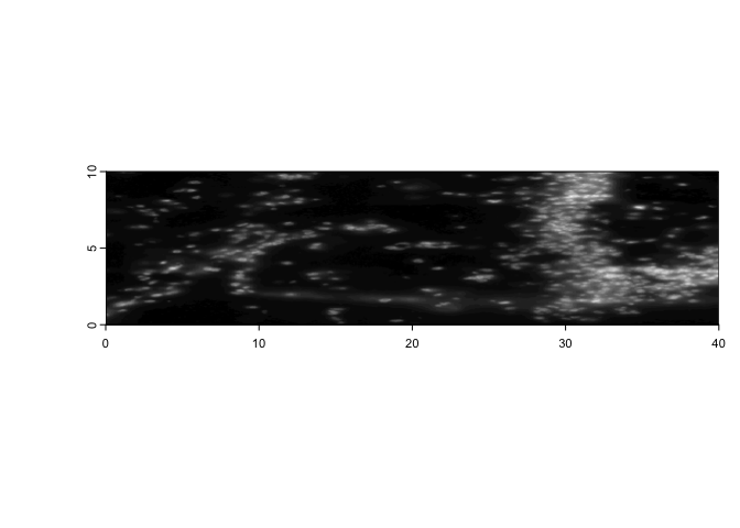
ext(image) <- e # replace
6 Spatial Transformations#
Commonly used spatial transformations are coordinate translations,
flips, and rotations. Giotto extends generics from terra through the
use of spatShift() (shift() in terra), flip(), and
spin() respectively.
6.1 coordinate translation#
spatShift() is used for simple coordinate translations. It takes the
params dx and dy for distance to translate along either axis.
plot(spat_locs)
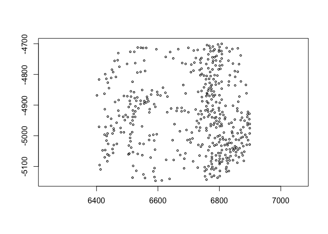
plot(spatShift(spat_locs, dx = 5e3))
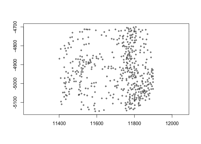
(pay attention to the x coords)
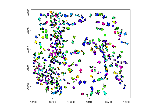
6.2 flip#
flip() will flip the data over a defined line of either ‘vertical’
or ‘horizontal’ symmetry (default is ‘vertical’ with the line of
symmetry being y = 0. The direction param partial matches for
either ‘vertical’ or ‘horizontal’. The y0 and x0 params define
where the line of symmetry is.y0 or x0 param.rb = getRainbowColors(100)
plot(gpoly, col = rb)
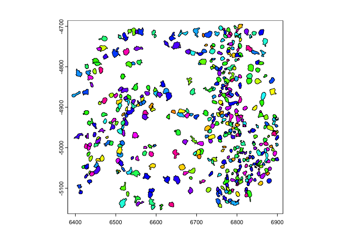
plot(flip(gpoly), col = rb) # flip to positive y
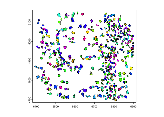
plot(flip(gpoly, direction = 'h', x0 = 1e4), col = rb) # flip across x = 10000
6.3 spin#
spin() allows rotating of vector data through degrees passed to
angle param. The rotation happens about a coordinate defined by
x0 and y0. By default x0 and y0 are defined as the
object center.
plot(gpoints)
plot(spin(gpoints, angle = 45))
plot(spin(gpoints, angle = 45, x0 = 0, y0 = 0))

7 Session Info#
sessionInfo()
R version 4.2.1 (2022-06-23)
Platform: x86_64-apple-darwin17.0 (64-bit)
Running under: macOS Big Sur ... 10.16

Matrix products: default
BLAS:   /Library/Frameworks/R.framework/Versions/4.2/Resources/lib/libRblas.0.dylib
LAPACK: /Library/Frameworks/R.framework/Versions/4.2/Resources/lib/libRlapack.dylib

locale:
[1] en_US.UTF-8/en_US.UTF-8/en_US.UTF-8/C/en_US.UTF-8/en_US.UTF-8

attached base packages:
[1] stats     graphics  grDevices utils     datasets  methods   base

other attached packages:
[1] GiottoData_0.2.3 Giotto_3.3.1

loaded via a namespace (and not attached):
 [1] Rcpp_1.0.11       pillar_1.9.0      compiler_4.2.1    tools_4.2.1
 [5] digest_0.6.31     scattermore_0.8   checkmate_2.2.0   jsonlite_1.8.4
 [9] evaluate_0.21     lifecycle_1.0.3   tibble_3.2.1      gtable_0.3.3
[13] lattice_0.20-45   png_0.1-8         pkgconfig_2.0.3   rlang_1.1.1
[17] igraph_1.4.2      Matrix_1.5-4      cli_3.6.1         rstudioapi_0.14
[21] parallel_4.2.1    yaml_2.3.7        xfun_0.39         fastmap_1.1.1
[25] terra_1.7-39      withr_2.5.0       dplyr_1.1.2       knitr_1.42
[29] generics_0.1.3    vctrs_0.6.2       rprojroot_2.0.3   grid_4.2.1
[33] tidyselect_1.2.0  here_1.0.1        reticulate_1.28   glue_1.6.2
[37] data.table_1.14.8 R6_2.5.1          fansi_1.0.4       rmarkdown_2.21
[41] ggplot2_3.4.2     magrittr_2.0.3    backports_1.4.1   scales_1.2.1
[45] codetools_0.2-18  htmltools_0.5.5   colorspace_2.1-0  utf8_1.2.3
[49] munsell_0.5.0