Spatial genes detection with binSpect#
- Date:
4/7/23
1. Load the pre-processed mini visium dataset#
This dataset is a subset of the Visium 10X mouse brain dataset. It has been fully processed and is easily available through the GiottoData package.
# Ensure Giotto Suite is installed
if(!"Giotto" %in% installed.packages()) {
  devtools::install_github("drieslab/Giotto@suite")
}
library(Giotto)

# Ensure Giotto Data is installed
if(!"GiottoData" %in% installed.packages()) {
  devtools::install_github("drieslab/GiottoData")
}
library(GiottoData)

# Ensure the Python environment for Giotto has been installed
genv_exists = checkGiottoEnvironment()
if(!genv_exists){
  # The following command need only be run once to install the Giotto environment
  installGiottoEnvironment()
}
visium = loadGiottoMini(dataset = 'visium')
The binSpect method identifies genes with a spatial coherent expression pattern based on binarization of individual cells/spots and the underlying spatial network. Here we will first create two different types of spatial networks and identify and visualize the top detected genes.
2. Create spatial network#
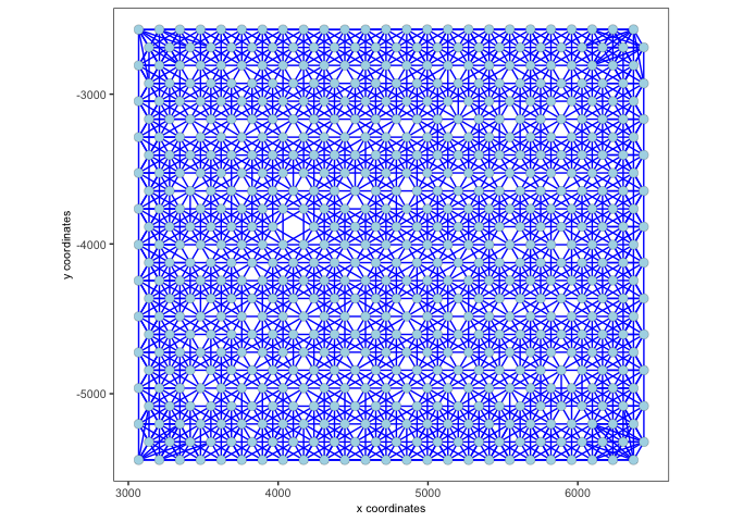
2.1 Default network#
The default network is a Delaunay network.
visium <- createSpatialNetwork(gobject = visium)

spatPlot2D(gobject = visium,
           show_network= T,
           network_color = 'blue')
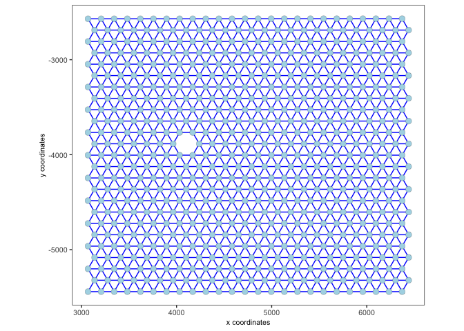
2.2 Custom network#
A custom spatial network can be created based on k (number of spatial neighbors) and / or maximum distance.
visium <- createSpatialNetwork(gobject = visium,
                               method = 'kNN', k = 10,
                               maximum_distance_knn = 400,
                               name = 'spatial_network')

spatPlot2D(gobject = visium,
           show_network= T,
           network_color = 'blue',
           spatial_network_name = 'spatial_network')
3. Run spatial gene expression test#
showGiottoSpatNetworks(visium)
└──Spatial unit "cell"
   ├──S4 spatialNetworkObj "Delaunay_network"   (1770 rows)
   │                      from                 to sdimx_begin sdimy_begin sdimx_end
   │     1: AAAGGGATGTAGCAAG-1 TCAAACAACCGCGTCG-1        5477       -4125      5340
   │     2: AAAGGGATGTAGCAAG-1 ACGATCATACATAGAG-1        5477       -4125      5546
   │     3: AAAGGGATGTAGCAAG-1 TATGCTCCCTACTTAC-1        5477       -4125      5408
   │     4: AAAGGGATGTAGCAAG-1 TTGTTCAGTGTGCTAC-1        5477       -4125      5615
   │        sdimy_end distance      weight
   │     1:     -4125 137.0000 0.007299270
   │     2:     -4244 137.5573 0.007269700
   │     3:     -4244 137.5573 0.007269700
   │     4:     -4125 138.0000 0.007246377
   │
   └──S4 spatialNetworkObj "spatial_network"   (3288 rows)
                          from                 to sdimx_begin sdimy_begin sdimx_end
         1: AAAGGGATGTAGCAAG-1 TCAAACAACCGCGTCG-1        5477       -4125      5340
         2: AAAGGGATGTAGCAAG-1 ACGATCATACATAGAG-1        5477       -4125      5546
         3: AAAGGGATGTAGCAAG-1 TATGCTCCCTACTTAC-1        5477       -4125      5408
         4: AAAGGGATGTAGCAAG-1 TTGTTCAGTGTGCTAC-1        5477       -4125      5615
            sdimy_end distance      weight
         1:     -4125 137.0000 0.007246377
         2:     -4244 137.5573 0.007217233
         3:     -4244 137.5573 0.007217233
         4:     -4125 138.0000 0.007194245
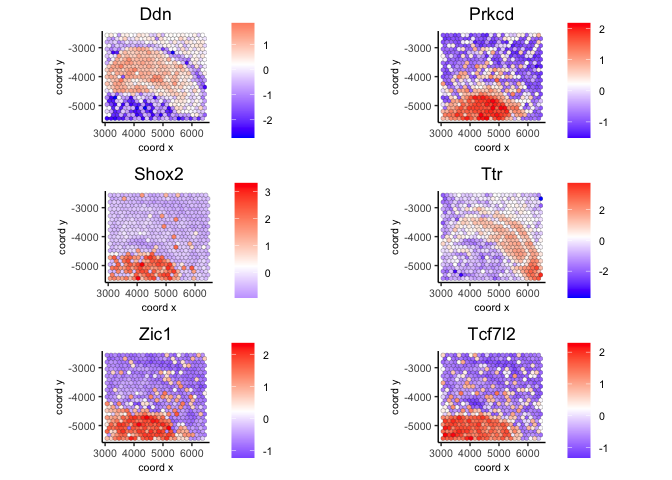
3.1 Use kNN network#
ranktest = binSpect(visium, bin_method = 'rank',
                    calc_hub = T, hub_min_int = 5,
                    spatial_network_name = 'spatial_network')
This is the single parameter version of binSpect
1. matrix binarization complete

2. spatial enrichment test completed

3. (optional) average expression of high expressing cells calculated

4. (optional) number of high expressing cells calculated
spatFeatPlot2D(visium,
               expression_values = 'scaled',
               feats = ranktest$feats[1:6], cow_n_col = 2, point_size = 1.5)
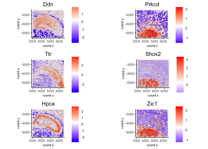
3.2 Use delaunay network#
ranktest_delaunay = binSpect(visium, bin_method = 'rank',
                    calc_hub = T, hub_min_int = 5,
                    spatial_network_name = 'Delaunay_network')
This is the single parameter version of binSpect
1. matrix binarization complete

2. spatial enrichment test completed

3. (optional) average expression of high expressing cells calculated

4. (optional) number of high expressing cells calculated
spatFeatPlot2D(visium,
               expression_values = 'scaled',
               feats = ranktest_delaunay$feats[1:6], cow_n_col = 2, point_size = 1.5)
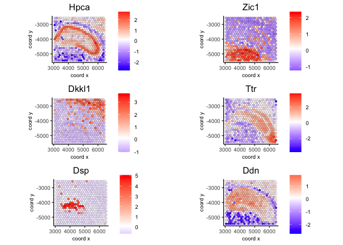
3.3 Use handpicked genes from top 50 genes#
spatFeatPlot2D(visium,
               expression_values = 'scaled',
               feats = c('Hpca', 'Zic1', 'Dkkl1', 'Ttr', 'Dsp', 'Ddn'),
               cow_n_col = 2, point_size = 1.5)
Session Info#
sessionInfo()
R version 4.2.1 (2022-06-23)
Platform: x86_64-apple-darwin17.0 (64-bit)
Running under: macOS Big Sur ... 10.16

Matrix products: default
BLAS:   /Library/Frameworks/R.framework/Versions/4.2/Resources/lib/libRblas.0.dylib
LAPACK: /Library/Frameworks/R.framework/Versions/4.2/Resources/lib/libRlapack.dylib

locale:
[1] en_US.UTF-8/en_US.UTF-8/en_US.UTF-8/C/en_US.UTF-8/en_US.UTF-8

attached base packages:
[1] stats     graphics  grDevices utils     datasets  methods   base

other attached packages:
[1] GiottoData_0.2.1 Giotto_3.2

loaded via a namespace (and not attached):
 [1] Rcpp_1.0.10       pillar_1.9.0      compiler_4.2.1    tools_4.2.1
 [5] digest_0.6.31     jsonlite_1.8.4    evaluate_0.20     lifecycle_1.0.3
 [9] tibble_3.2.1      gtable_0.3.3      lattice_0.20-45   png_0.1-8
[13] pkgconfig_2.0.3   rlang_1.1.0       igraph_1.4.1      Matrix_1.5-3
[17] cli_3.6.1         rstudioapi_0.14   parallel_4.2.1    yaml_2.3.7
[21] xfun_0.37         fastmap_1.1.1     terra_1.7-3       withr_2.5.0
[25] dplyr_1.1.1       knitr_1.42        generics_0.1.3    vctrs_0.6.1
[29] cowplot_1.1.1     grid_4.2.1        tidyselect_1.2.0  reticulate_1.28
[33] glue_1.6.2        data.table_1.14.8 R6_2.5.1          fansi_1.0.4
[37] rmarkdown_2.20    farver_2.1.1      deldir_1.0-6      ggplot2_3.4.1
[41] magrittr_2.0.3    scales_1.2.1      codetools_0.2-19  htmltools_0.5.4
[45] colorspace_2.1-0  labeling_0.4.2    utf8_1.2.3        munsell_0.5.0
[49] dbscan_1.1-11