Nanostring CosMx Subcellular Lung Cancer#
- Date:
Compiled 2022-11-30
This example uses subcellular data from Nanostring’s CosMx Spatial Molecular Imager. This publicly available dataset is from an FFPE sample of non-small-cell lung cancer (NSCLC). This example works with Lung12.
# Ensure Giotto Suite is installed.
if(!"Giotto" %in% installed.packages()) {
  devtools::install_github("drieslab/Giotto@suite")
}
library(Giotto)

# Ensure the Python environment for Giotto has been installed.
genv_exists = checkGiottoEnvironment()
if(!genv_exists){
  # The following command need only be run once to install the Giotto environment.
  installGiottoEnvironment()
}
1. Setup#
# Custom color palettes from rcartocolor
# pal10 = rcartocolor::carto_pal(n = 10, name = 'Pastel')
pal10 = c("#66C5CC","#F6CF71","#F89C74","#DCB0F2","#87C55F",
          "#9EB9F3","#FE88B1","#C9DB74","#8BE0A4","#B3B3B3")
# viv10 = rcartocolor::carto_pal(n = 10, name = 'Vivid')
viv10 = c("#E58606","#5D69B1","#52BCA3","#99C945","#CC61B0",
          "#24796C","#DAA51B","#2F8AC4","#764E9F","#A5AA99")

# set working directory
results_folder = '/path/to/directory'

# Optional: Specify a path to a Python executable within a conda or miniconda
# environment. If set to NULL (default), the Python executable within the previously
# installed Giotto environment will be used.
my_python_path = NULL # alternatively, "/local/python/path/python" if desired.

## Set object behavior
# by directly saving plots, but not rendering them you will save a lot of time
instrs = createGiottoInstructions(save_dir = results_folder,
                                  save_plot = TRUE,
                                  show_plot = FALSE,
                                  return_plot = FALSE,
                                  python_path = my_python_path)
1.1 CosMx Project loading function#
giotto object with giottoPoints objects for both ‘rna’ and
‘neg_probe’ nested in the gobject feat_info slot, and a
giottoPolygon object for the ‘cell’ spatial unit in the
spatial_info slot.Additionally, a comparison of the count matrix produced through the convenience function ‘subcellular’ workflow and Nanostring’s provided matrix can be found at Section 6.4.
## provide path to nanostring folder
data_path = '/path/to/data/Lung12-Flat_files_and_images/'

## create giotto cosmx object
fov_join = createGiottoCosMxObject(cosmx_dir = data_path,
                                   data_to_use = 'subcellular', # only subcellular
                                   FOVs = c(2,3,4),
                                   instructions = instrs)

showGiottoFeatInfo(fov_join)
showGiottoSpatialInfo(fov_join)
2. Data exploration and loading#
2.1 Subcellular detections (points info)#
tx_file.csv contains the subcellular detections information. It
contains information on each of the individual feature detections
within the sample.## provide path to nanostring folder
data_path = '/path/to/data/Lung12-Flat_files_and_images/'
# load transcript coordinates
tx_coord_all = data.table::fread(paste0(data_path, 'Lung12_tx_file.csv'))
colnames(tx_coord_all)
cat('\n')
# z planes
tx_coord_all[, table(z)]
cat('\n')
# Cell compartment
tx_coord_all[, table(CellComp)]
# [1] "fov"         "cell_ID"     "x_global_px" "y_global_px"
# [5] "x_local_px"  "y_local_px"  "z"           "target"
# [9] "CellComp"
#
# z
#      -1       0       1       2       3       4       5       6
#   23723 3466178 2522315 2694973 2686531 2648926 2660346 2711105
#       7       8       9      10      11      12      13      14
# 2855259 3700831   36840    6594    6466    6787    6944    6959
#      15      16
#   17603       2
#
# CellComp
#         0 Cytoplasm  Membrane   Nuclear
#   6619744   5770549   3368411  10299678
2.2 Split detections by features vs negative probes#
tx_file.csv contains information on both actual features (960
targeted gene probes in this dataset) and negative probes (20) that
are targeted to alien sequences defined by the External RNA Controls
Consortium (ERCC) that do not exist in human tissue.feat_type) and placed in separate expression matrices.all_IDs = tx_coord_all[, unique(target)]
# negative probe IDs
neg_IDs = all_IDs[grepl(pattern = 'NegPrb', all_IDs)]
cat('Negative Probe IDs\n')
neg_IDs
cat('\nFeature IDs\n')
feat_IDs = all_IDs[!all_IDs %in% neg_IDs]
length(feat_IDs)
# split detections
feat_coords_all = tx_coord_all[target %in% feat_IDs]
neg_coords_all = tx_coord_all[target %in% neg_IDs]
cat('\nFeatures: ', feat_coords_all[, .N], '\n',
'NegProbes: ', neg_coords_all[, .N])
# Negative Probe IDs
#  [1] "NegPrb15" "NegPrb18" "NegPrb7"  "NegPrb21" "NegPrb13"
#  [6] "NegPrb10" "NegPrb11" "NegPrb9"  "NegPrb3"  "NegPrb16"
# [11] "NegPrb23" "NegPrb14" "NegPrb20" "NegPrb8"  "NegPrb19"
# [16] "NegPrb6"  "NegPrb5"  "NegPrb12" "NegPrb17" "NegPrb22"
#
# Number of feature IDs
# [1] 960
#
# Features:  25875734
# NegProbes:  182648
feat_IDs
#   [1] "IL7R"       "SEC61G"     "IGHA1"      "CD164"      "IL6"
#   [6] "CCR2"       "KRT86"      "NEAT1"      "NLRP1"      "S100A10"
#  [11] "KRT80"      "MYH11"      "OLR1"       "FYN"        "NR1H4"
#  [16] "NDRG1"      "AGR2"       "FGR"        "NFKB1"      "IL4R"
#  [21] "VWF"        "EOMES"      "COL16A1"    "IL1RL1"     "ITGAL"
#  [26] "GLUD1"      "STAT3"      "MAPK14"     "VHL"        "CD44"
#  [31] "RAMP1"      "ZFP36"      "CD27"       "GDF15"      "EPCAM"
#  [36] "LAMP3"      "LTB"        "COL12A1"    "LGALS9"     "HLA-DQB1"
#  [41] "CLU"        "ALCAM"      "TLR7"       "FGF1"       "NR1H3"
#  [46] "TNFSF18"    "EIF5A"      "LGALS3"     "CD63"       "FOXP3"
#  [51] "DCN"        "CUZD1"      "LIF"        "BMP6"       "HCST"
#  [56] "VSIR"       "STAT1"      "GDNF"       "UBE2C"      "APOA1"
#  [61] "ADGRF1"     "PDGFC"      "IL17A"      "YES1"       "TGFBR2"
#  [66] "GPX3"       "IFIH1"      "SOX9"       "MX1"        "IGKC"
#  [71] "CD8A"       "PTGES3"     "KRAS"       "CRYAB"      "ACTA2"
#  [76] "EGF"        "CD5L"       "BCL2L1"     "SRGN"       "FGFR3"
#  [81] "CD53"       "CELSR2"     "MTRNR2L1"   "LAMP2"      "LAIR1"
#  [86] "FGF13"      "EFNA1"      "CLEC2B"     "FZD5"       "SYK"
#  [91] "FES"        "MZT2A"      "SERPINA1"   "HIF1A"      "JUN"
#  [96] "THBS1"      "CHEK2"      "CD274"      "CXCL3"      "IL11"
# [101] "GPX1"       "FASLG"      "EPHA2"      "TGFB3"      "RARG"
# [106] "CLDN4"      "G6PC2"      "KITLG"      "ADGRG3"     "RPL34"
# [111] "HLA-A"      "ESAM"       "HDAC1"      "MGP"        "MECOM"
# [116] "MRC2"       "ACE2"       "COL4A2"     "CDH1"       "ATG10"
# [121] "IL32"       "SERPINA3"   "SRC"        "IGFBP6"     "IER3"
# [126] "QRFPR"      "CD276"      "ITGA9"      "INHBA"      "CXCL1"
# [131] "ATG12"      "ERBB2"      "FCRLA"      "TIE1"       "EFNB1"
# [136] "IGHG2"      "FZD3"       "SAA1"       "CCL23"      "JUNB"
# [141] "COTL1"      "CSF1R"      "TNFAIP6"    "KIT"        "RSPO1"
# [146] "RARB"       "CXCR4"      "CD28"       "FGFR2"      "RGS1"
# [151] "ACVR2A"     "CD3G"       "ADORA2A"    "IGFBP3"     "NOD2"
# [156] "KRT1"       "LPAR5"      "CD36"       "ACKR3"      "CCL3"
# [161] "CD48"       "TYK2"       "TGFB1"      "CD2"        "CTSG"
# [166] "CFLAR"      "IDO1"       "TIMP1"      "TGFBR1"     "BTK"
# [171] "BMP7"       "HSPB1"      "GDF10"      "CD37"       "ADIPOQ"
# [176] "WNT5A"      "TAP1"       "CRIP1"      "ATF3"       "PTHLH"
# [181] "ITGA3"      "CD3E"       "TGFB2"      "HLA-DRA"    "TLR8"
# [186] "ADGRG5"     "ITGAE"      "MKI67"      "EPHA4"      "CSF3"
# [191] "BMP3"       "COL6A1"     "IL1RN"      "CCR7"       "CD19"
# [196] "VCAN"       "FAS"        "WNT7A"      "FCGBP"      "IL18R1"
# [201] "EPHB4"      "TYROBP"     "KRT14"      "TACSTD2"    "PF4"
# [206] "JCHAIN"     "WIF1"       "ANXA2"      "CYSTM1"     "RPL32"
# [211] "KRT13"      "CFD"        "COL14A1"    "STMN1"      "CCL4"
# [216] "PTGS2"      "SUCNR1"     "RAD51"      "THBS2"      "KDR"
# [221] "SCGB3A1"    "CENPF"      "CD52"       "ROR1"       "GZMA"
# [226] "HCAR2"      "CSF3R"      "IL10RB"     "CXCL2"      "GZMH"
# [231] "PECAM1"     "CCL2"       "DUSP5"      "SLC40A1"    "PTGDR2"
# [236] "ITGB8"      "SAT1"       "S100A6"     "IFNB1"      "IGFBP7"
# [241] "TCL1A"      "S100P"      "DST"        "IFI27"      "H4C3"
# [246] "MMP16"      "CX3CL1"     "CALM3"      "DUSP6"      "IL36G"
# [251] "COL6A2"     "SOX4"       "TNFRSF10B"  "CCL19"      "KRT19"
# [256] "ACE"        "TPM2"       "FGF9"       "COL1A2"     "RAC1"
# [261] "RPL21"      "IL15RA"     "HMGN2"      "VEGFA"      "CDKN1A"
# [266] "COL18A1"    "IGF1"       "SLPI"       "FLT1"       "CD9"
# [271] "KRT5"       "TNFRSF12A"  "MIF"        "YBX3"       "S100A4"
# [276] "HPGDS"      "INHA"       "IGHG1"      "CLEC12A"    "NPPC"
# [281] "KRT8"       "IFNL2"      "TPSAB1"     "ATR"        "SMAD3"
# [286] "TUBB"       "KRT7"       "TBX21"      "CTNNB1"     "IRF4"
# [291] "DMBT1"      "ACKR4"      "SPARCL1"    "POU5F1"     "IRF3"
# [296] "MMP7"       "RXRA"       "TNFRSF11B"  "IL12A"      "DDR1"
# [301] "IL1RAP"     "ITGAM"      "DDIT3"      "TWIST1"     "NLRP2"
# [306] "LDLR"       "CXCL10"     "SAA2"       "KRT23"      "CAV1"
# [311] "IL1A"       "B2M"        "ELANE"      "TEK"        "ITGAV"
# [316] "FKBP11"     "ICAM3"      "TNFSF10"    "ERBB3"      "ADGRG6"
# [321] "CD80"       "CPA3"       "CTSW"       "MAML2"      "PHLDA2"
# [326] "LIFR"       "IL13RA1"    "HILPDA"     "KLF2"       "EPHA7"
# [331] "IL18"       "COL1A1"     "GLUL"       "DDR2"       "TM4SF1"
# [336] "KRT6C"      "COL5A2"     "CLEC10A"    "CSHL1"      "IL2RB"
# [341] "TPSB2"      "ITK"        "C1QC"       "CXCL16"     "IFNA1"
# [346] "IFNAR1"     "IGF2"       "ATG5"       "NKG7"       "RARRES2"
# [351] "AZU1"       "CLEC4A"     "GSTP1"      "GPBAR1"     "TNFRSF1A"
# [356] "IFITM3"     "DUSP1"      "CCR10"      "EPHB2"      "ITGA6"
# [361] "CAMP"       "CD14"       "TXK"        "SERPINH1"   "NPR3"
# [366] "MTOR"       "CRP"        "MMP2"       "IGF2R"      "TAGLN"
# [371] "PSAP"       "MS4A1"      "MST1R"      "KLRK1"      "BGN"
# [376] "TNFRSF9"    "P2RY12"     "PTK2"       "IL23A"      "RXRB"
# [381] "NOTCH3"     "FOXF1"      "COL15A1"    "SQSTM1"     "CCL15"
# [386] "S100A2"     "MMP3"       "CCL8"       "ESR1"       "SMARCB1"
# [391] "RGCC"       "PPARA"      "IL2RA"      "SMAD4"      "EFNA4"
# [396] "RARRES1"    "COL3A1"     "ITGB6"      "CD74"       "ANXA4"
# [401] "SFN"        "ARHGDIB"    "TNFRSF10A"  "VEGFC"      "HLA-B"
# [406] "HLA-DRB5"   "CD3D"       "ITGA1"      "ANGPT1"     "KRT24"
# [411] "MET"        "MALAT1"     "HSP90AB1"   "ABL2"       "LTF"
# [416] "MMP12"      "ACKR1"      "MERTK"      "S100A9"     "FZD8"
# [421] "INS"        "CD33"       "HDAC3"      "OSM"        "CYP1B1"
# [426] "ITGB2"      "CD40LG"     "CALD1"      "CLOCK"      "COL11A1"
# [431] "C9orf16"    "IL1B"       "CCL11"      "FGF18"      "BID"
# [436] "MT1X"       "KLK3"       "CCL28"      "RAMP3"      "OXER1"
# [441] "IL3RA"      "ADGRB3"     "FASN"       "MMP8"       "ITGA2"
# [446] "CCL5"       "MRC1"       "IGFBP5"     "PPARG"      "G6PD"
# [451] "CCND1"      "TLR2"       "RAMP2"      "PTPRC"      "BIRC5"
# [456] "ITM2A"      "IL11RA"     "STAT5A"     "COL27A1"    "PPARD"
# [461] "FFAR4"      "ADGRE5"     "FGF7"       "MMP14"      "MZB1"
# [466] "NOSIP"      "TNFRSF19"   "ADGRL2"     "FABP5"      "IFNGR1"
# [471] "VTN"        "FCER1G"     "CASP8"      "ITGB1"      "SOX2"
# [476] "GNLY"       "CCRL2"      "RSPO3"      "IGF1R"      "NOTCH2"
# [481] "IL10RA"     "TWIST2"     "LMNA"       "LCN2"       "PSCA"
# [486] "ADGRG2"     "AKT1"       "SPRY4"      "SELL"       "PDGFD"
# [491] "LYN"        "WNT11"      "IFNAR2"     "TNFRSF14"   "OASL"
# [496] "SNAI2"      "OLFM4"      "CYTOR"      "CXCR6"      "RARA"
# [501] "RUNX3"      "WNT3"       "PIGR"       "PDCD1"      "RGS2"
# [506] "LEFTY2"     "TLR5"       "CDKN3"      "ACVRL1"     "FZD4"
# [511] "FGF2"       "SMO"        "AHR"        "SELPLG"     "HDAC5"
# [516] "GATA3"      "CD81"       "PNOC"       "PLAC8"      "HLA-DPA1"
# [521] "MXRA8"      "CXCR1"      "SNAI1"      "KLRB1"      "IFNG"
# [526] "COL17A1"    "IL7"        "LUM"        "MMP1"       "IL22RA1"
# [531] "ITGB5"      "IL33"       "LYZ"        "FFAR3"      "SOD2"
# [536] "HCK"        "CCR1"       "UCP1"       "WNT10B"     "OXGR1"
# [541] "FGG"        "BST1"       "RELT"       "WNT5B"      "IL12RB2"
# [546] "DUSP2"      "HBB"        "CD83"       "CLEC2D"     "CSF2RB"
# [551] "HDAC11"     "IL17RE"     "COL5A3"     "WNT7B"      "TSLP"
# [556] "CALM1"      "IL2RG"      "CLEC4D"     "ADGRL1"     "APP"
# [561] "KRT20"      "CCL4L2"     "CD68"       "VIM"        "H2AZ1"
# [566] "LINC02446"  "BAX"        "CD34"       "FZD6"       "CEACAM6"
# [571] "ST6GALNAC3" "PTGS1"      "TNFSF8"     "VEGFD"      "ADGRF5"
# [576] "HSD3B2"     "COL9A2"     "KRT16"      "PDGFB"      "FYB1"
# [581] "CASP3"      "BRCA1"      "CXCL9"      "CLEC1A"     "IL20RA"
# [586] "HSPA1B"     "LEP"        "GCG"        "LY6D"       "DUSP4"
# [591] "CD59"       "EPHA3"      "RORA"       "WNT2"       "ADGRA2"
# [596] "CALM2"      "CLEC7A"     "HLA-C"      "TNFSF4"     "TYMS"
# [601] "IFITM1"     "MT2A"       "SMAD2"      "KRT17"      "PTK6"
# [606] "OSMR"       "CHEK1"      "CD79A"      "CASR"       "SPRY2"
# [611] "IGHM"       "S100B"      "GDF6"       "TNFSF9"     "IL34"
# [616] "DLL1"       "SPOCK2"     "NRXN1"      "CSF1"       "IL6ST"
# [621] "HDAC4"      "TOP2A"      "GAS6"       "ITGA5"      "COL5A1"
# [626] "ST6GAL1"    "TNFRSF1B"   "EMP3"       "TNFRSF13B"  "KRT6B"
# [631] "ABL1"       "CTLA4"      "EPOR"       "SLC2A4"     "MMP9"
# [636] "IL24"       "CHI3L1"     "PTGDS"      "CD209"      "RPL37"
# [641] "CD38"       "GPNMB"      "STAT5B"     "ETS1"       "DDC"
# [646] "LGALS1"     "KRT18"      "MYL9"       "EFNB3"      "ANXA1"
# [651] "BST2"       "COL4A1"     "GSN"        "CD58"       "CD55"
# [656] "PTPRCAP"    "VCAM1"      "ACVR1"      "IL12B"      "RB1"
# [661] "C11orf96"   "XCL2"       "SPINK1"     "C1QA"       "ITGAX"
# [666] "TNFRSF21"   "JAK1"       "IL17RB"     "IFNL3"      "HLA-DQA1"
# [671] "ETV5"       "TNFSF12"    "TIGIT"      "ENTPD1"     "RSPO2"
# [676] "ANGPT4"     "TLR4"       "EPHB3"      "ICOSLG"     "NRIP3"
# [681] "MARCO"      "NLRC4"      "CCL13"      "CIITA"      "OAS1"
# [686] "HBA1"       "EFNB2"      "HLA-DRB1"   "ADGRF3"     "TUBB4B"
# [691] "MAF"        "TSHZ2"      "SPP1"       "IL2"        "CALB1"
# [696] "CCL7"       "ADGRE1"     "XCL1"       "PDGFRA"     "CXCL17"
# [701] "STAT6"      "SLC2A1"     "COL8A1"     "SST"        "PTGES"
# [706] "LAG3"       "CCL18"      "CIDEA"      "BMP4"       "CXCL8"
# [711] "EGFR"       "KRT4"       "DNMT3A"     "FLT3LG"     "HLA-E"
# [716] "FZD7"       "OAS3"       "COL9A3"     "TLR1"       "APOD"
# [721] "ICAM2"      "PDGFA"      "PRF1"       "TFEB"       "AREG"
# [726] "ARG1"       "IL27RA"     "TNFRSF10D"  "GADD45B"    "HSP90AA1"
# [731] "DPP4"       "MMP19"      "TPM1"       "P2RX5"      "CST7"
# [736] "BEST1"      "MMP10"      "CXCR5"      "PTTG1"      "TOX"
# [741] "CDH11"      "MYC"        "PDGFRB"     "ANGPTL1"    "ADGRF4"
# [746] "AHI1"       "HLA-DPB1"   "TNFRSF11A"  "TNFSF15"    "AR"
# [751] "IL1R1"      "CCL20"      "NLRC5"      "HAVCR2"     "LTBR"
# [756] "GDF3"       "TAP2"       "INSR"       "IL15"       "HSD17B2"
# [761] "CD84"       "MPO"        "SELENOP"    "SEC23A"     "DHRS2"
# [766] "HSP90B1"    "HSPA1A"     "BCL2"       "XBP1"       "RBPJ"
# [771] "EZH2"       "MSMB"       "EFNA5"      "AXL"        "NLRP3"
# [776] "FN1"        "CD8B"       "CXCR2"      "CNTFR"      "TNFRSF18"
# [781] "COL6A3"     "CCR5"       "NRG4"       "ITGB4"      "CSF2"
# [786] "TLR3"       "IGHD"       "CD70"       "INHBB"      "MAPK13"
# [791] "MEG3"       "PLA2R1"     "MAP1LC3B"   "PPBP"       "IL17D"
# [796] "CD4"        "IL20"       "IL17B"      "KRT15"      "RPL22"
# [801] "RYK"        "NTRK2"      "CCL21"      "DDX58"      "CD24"
# [806] "IL10"       "PARP1"      "CD300A"     "CDH5"       "BTG1"
# [811] "NFKBIA"     "PRSS2"      "CXCL6"      "CSF2RA"     "ADGRD1"
# [816] "WNT9A"      "ADIRF"      "ICOS"       "KRT6A"      "CD86"
# [821] "C5AR2"      "FOS"        "SCG5"       "IFNGR2"     "LGALS3BP"
# [826] "CD69"       "RGS5"       "BMP2"       "BMP5"       "RELA"
# [831] "CLCF1"      "COL4A5"     "BMPR2"      "FCGR3A"     "REG1A"
# [836] "EZR"        "IL12RB1"    "RAC2"       "C1QB"       "RNF43"
# [841] "CLEC4E"     "PCNA"       "CLEC5A"     "FABP4"      "PGR"
# [846] "CD163"      "ICAM1"      "ADGRG1"     "HTT"        "CD47"
# [851] "AQP3"       "OAS2"       "GPR183"     "LEFTY1"     "WNT2B"
# [856] "BMX"        "JAG1"       "PTGIS"      "EPHB6"      "NPR2"
# [861] "SREBF1"     "CD40"       "DNTT"       "IL16"       "IFIT1"
# [866] "ANGPT2"     "PTGES2"     "DNMT1"      "GZMB"       "TSC22D1"
# [871] "HCAR3"      "FGF12"      "HGF"        "BMP1"       "ENG"
# [876] "CXCL5"      "B3GNT7"     "ADM2"       "CLEC14A"    "ARF1"
# [881] "ACVR1B"     "GC"         "AATK"       "ARTN"       "ADGRA3"
# [886] "FFAR2"      "TNF"        "S100A8"     "BATF3"      "SIGIRR"
# [891] "VPREB3"     "BECN1"      "FZD1"       "PROK2"      "NCR1"
# [896] "IL17RA"     "IL1R2"      "CPB1"       "JAK2"       "IL6R"
# [901] "NANOG"      "CYP19A1"    "NPPB"       "PGF"        "FPR1"
# [906] "NR1H2"      "NRXN3"      "NOTCH1"     "NR3C1"      "KRT10"
# [911] "SERPINB5"   "CSK"        "ADGRB2"     "CELSR1"     "GPER1"
# [916] "RPS4Y1"     "HMGB2"      "BMPR1A"     "PDCD1LG2"   "TNFRSF4"
# [921] "GZMK"       "FGFR1"      "GDF9"       "SOSTDC1"    "TNFSF14"
# [926] "NGFR"       "UPK3A"      "CCL3L3"     "BAG3"       "LY75"
# [931] "ADGRL4"     "TTR"        "NPR1"       "VEGFB"      "NRG1"
# [936] "AZGP1"      "PROKR1"     "CXCR3"      "STAT4"      "ETV4"
# [941] "ATM"        "TNFRSF17"   "APOB"       "ADGRE2"     "COL21A1"
# [946] "CX3CR1"     "CMKLR1"     "MS4A4A"     "COL9A1"     "TNFSF13B"
# [951] "SOD1"       "ACTG2"      "TP53"       "ADGRV1"     "IAPP"
# [956] "CCL26"      "CXCL14"     "CHGA"       "CXCL12"     "CEACAM1"
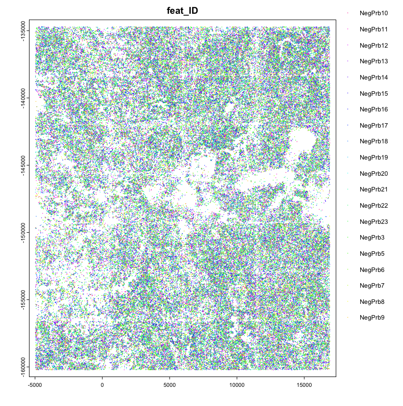
2.2.1 Preview negative probes (optional)#
giottoPoints and then using plot(). Here we show a preview of
the negative probes.feats param. The
default is to plot all points, which can be very slow for large data.neg_points = createGiottoPoints(
x = neg_coords_all[, .(target, x_global_px, y_global_px)]
)
plot(neg_points, point_size = 0.2, feats = neg_IDs)
2.3 FOV shifts#
fov_positions_file.csv contains information on the x and y shifts
needed in order to put the FOVs tiles together into a cohesive whole.
This information is needed during the image attachment and alignment
process.
#  load field of vision (fov) positions
fov_offset_file = data.table::fread(paste0(data_path, 'Lung12_fov_positions_file.csv'))
fov_offset_file
#     fov x_global_px y_global_px
#  1:   1  -4977.7778   -160233.3
#  2:   2    494.4444   -160233.3
#  3:   3   5966.6667   -160233.3
#  4:   4  11438.8889   -160233.3
#  5:   5  -4977.7778   -156583.3
#  6:   6    494.4444   -156583.3
#  7:   7   5966.6667   -156583.3
#  8:   8  11438.8889   -156583.3
#  9:   9  -4977.7778   -152933.3
# 10:  10    494.4444   -152933.3
# 11:  11   5966.6667   -152933.3
# 12:  12  11438.8889   -152933.3
# 13:  13  -4977.7778   -149283.3
# 14:  14    494.4444   -149283.3
# 15:  15   5966.6667   -149283.3
# 16:  16  11438.8889   -149283.3
# 17:  17  -4977.7778   -145633.3
# 18:  18    494.4444   -145633.3
# 19:  19   5966.6667   -145633.3
# 20:  20  11438.8889   -145633.3
# 21:  21  -4977.7778   -141983.3
# 22:  22    494.4444   -141983.3
# 23:  23   5966.6667   -141983.3
# 24:  24  11438.8889   -141983.3
# 25:  25  -4977.7778   -138333.3
# 26:  26    494.4444   -138333.3
# 27:  27   5966.6667   -138333.3
# 28:  28  11438.8889   -138333.3
#     fov x_global_px y_global_px
2.4 Choose field of view for analysis#
gobjects_list = list()

id_set = c('02', '03', '04')
3. Create a Giotto Object for each FOV#
for(fov_i in 1:length(id_set)) {

  fov_id = id_set[fov_i]


  # 1. original composite image as png
  original_composite_image = paste0(data_path, 'CellComposite/CellComposite_F0', fov_id,'.jpg')

  # 2. input cell segmentation as mask file
  segmentation_mask = paste0(data_path, 'CellLabels/CellLabels_F0', fov_id, '.tif')

  # 3. input features coordinates + offset
  feat_coord = feat_coords_all[fov == as.numeric(fov_id)]
  neg_coord = neg_coords_all[fov == as.numeric(fov_id)]
  feat_coord = feat_coord[,.(x_local_px, y_local_px, z, target)]
  neg_coord = neg_coord[,.(x_local_px, y_local_px, z, target)]
  colnames(feat_coord) = c('x', 'y', 'z', 'gene_id')
  colnames(neg_coord) = c('x', 'y', 'z', 'gene_id')
  feat_coord = feat_coord[,.(x, y, gene_id)]
  neg_coord = neg_coord[,.(x, y, gene_id)]


  fovsubset = createGiottoObjectSubcellular(
    gpoints = list('rna' = feat_coord,
                   'neg_probe' = neg_coord),
    gpolygons = list('cell' = segmentation_mask),
    polygon_mask_list_params = list(
      mask_method = 'guess',
      flip_vertical = TRUE,
      flip_horizontal = FALSE,
      shift_horizontal_step = FALSE
    ),
    instructions = instrs
  )


  # cell centroids are now used to provide the spatial locations
  fovsubset = addSpatialCentroidLocations(fovsubset,
                                          poly_info = 'cell')

  # create and add Giotto images
  composite = createGiottoLargeImage(raster_object = original_composite_image,
                                     negative_y = FALSE,
                                     name = 'composite')

  fovsubset = addGiottoImage(gobject = fovsubset,
                             largeImages = list(composite))


  fovsubset = convertGiottoLargeImageToMG(giottoLargeImage = composite,
                                          #mg_name = 'composite',
                                          gobject = fovsubset,
                                          return_gobject = TRUE)

  gobjects_list[[fov_i]] = fovsubset

}
4. Join FOV Giotto Objects#
new_names = paste0("fov0", id_set)

id_match = match(as.numeric(id_set), fov_offset_file$fov)
x_shifts = fov_offset_file[id_match]$x_global_px
y_shifts = fov_offset_file[id_match]$y_global_px

# Create Giotto object that includes all selected FOVs
fov_join = joinGiottoObjects(gobject_list = gobjects_list,
                             gobject_names = new_names,
                             join_method = 'shift',
                             x_shift = x_shifts,
                             y_shift = y_shifts)
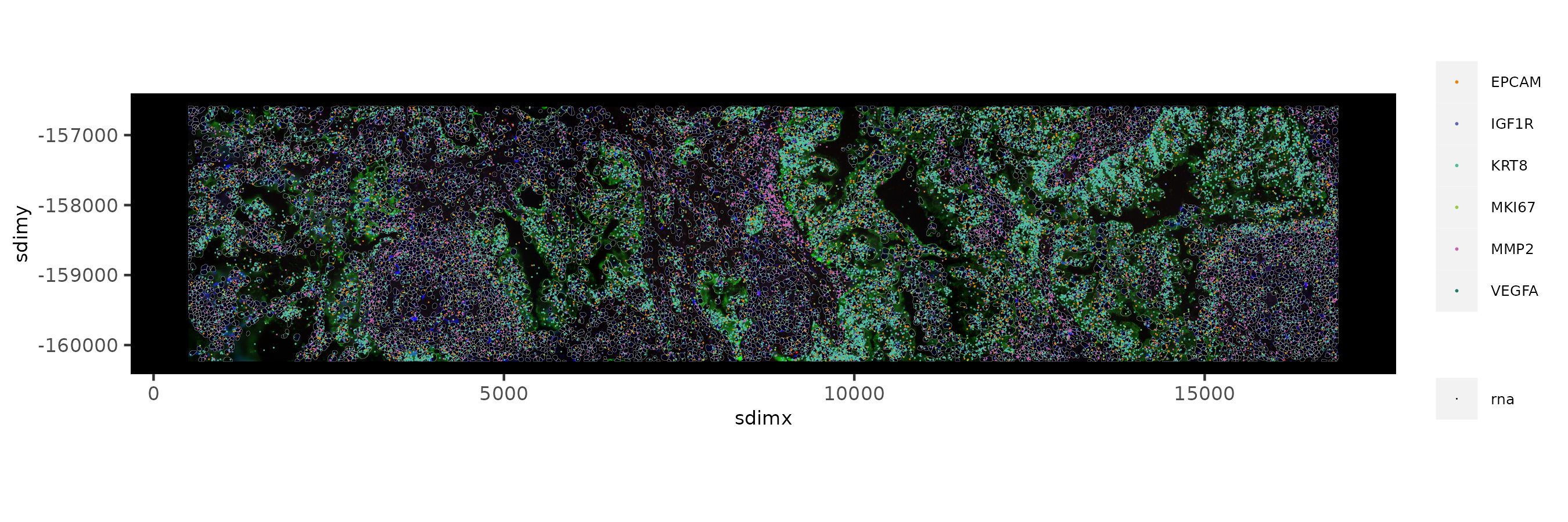
5. Visualize Cells and Genes of Interest#
When plotting subcellular data, Giotto uses the spatInSituPlot
functions. Spatial plots showing the feature points and polygons are
plotted using spatInSituPlotPoints().
showGiottoImageNames(fov_join)
# Set up vector of image names
id_set = c('02', '03', '04')
new_names = paste0("fov0", id_set)
image_names = paste0(new_names, '-image')
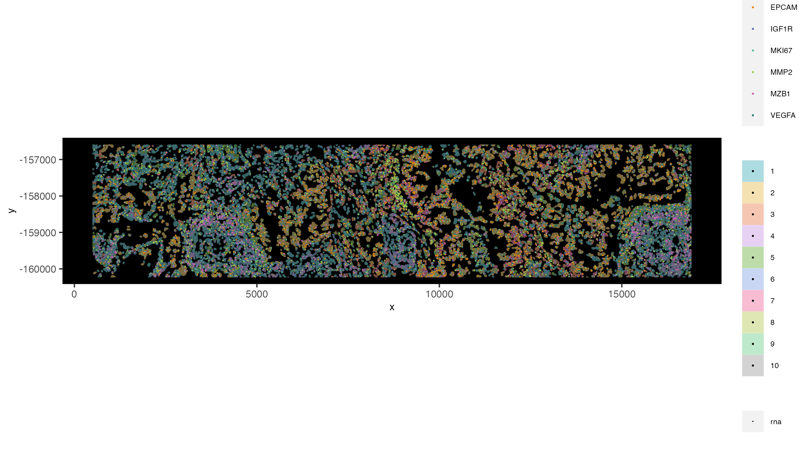
spatInSituPlotPoints(fov_join,
show_image = TRUE,
image_name = image_names,
feats = list('rna' = c('MMP2', 'VEGFA', 'IGF1R',
'MKI67', 'EPCAM', 'KRT8')),
feats_color_code = viv10,
spat_unit = 'cell',
point_size = 0.01,
show_polygon = TRUE,
use_overlap = FALSE,
polygon_feat_type = 'cell',
polygon_color = 'white',
polygon_line_size = 0.03,
save_param = list(base_height = 3,
save_name = '1_inSituFeats'))
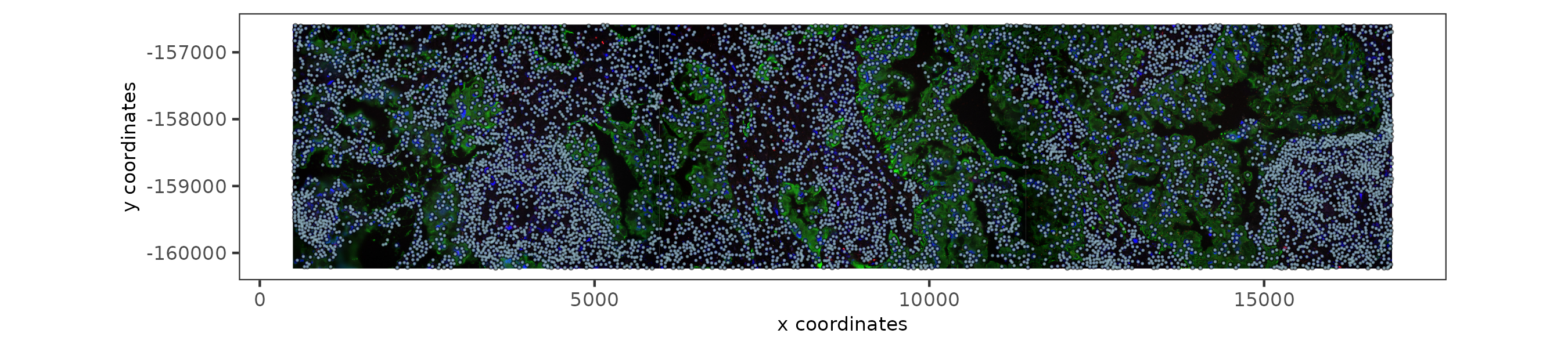
5.1 Visualize Cell Centroids#
The standard spatPlot2D() function can also be used, but this works
off only the aggregated information that is assembled based on the
subcellular information. Plotting information based on cell centroids
can be done through this function.
spatPlot2D(gobject = fov_join,
           image_name = image_names,
           show_image = TRUE,
           point_shape = 'no_border',
           point_size = 0.01,
           point_alpha = 0.5,
           coord_fix_ratio = 1,
           save_param = list(base_height = 2,
                             save_name = '2_spatCentroids'))
6. Aggregate subcellular features#
'cell'. This workflow is
recommended over loading the provided cell by feature (aggregated
expression) matrix and then including the subcellular information as
secondary data.'cell' and
the pre-generated aggregated information should be given a different
spatial unit such as 'cell_agg' to differentiate between the two
sources of information.\(~\)
In this step, we will be aggregating the feature points of 'rna' and
'neg_probe' into the 'cell' spatial unit.
# Find the feature points overlapped by polygons. This overlap information is then
# returned to the relevant giottoPolygon object's overlaps slot.
fov_join = calculateOverlapRaster(fov_join, feat_info = 'rna')
fov_join = calculateOverlapRaster(fov_join, feat_info = 'neg_probe')

# Convert the overlap information into a cell by feature expression matrix which
# is then stored in the Giotto object's expression slot
fov_join = overlapToMatrix(fov_join, feat_info = 'rna')
fov_join = overlapToMatrix(fov_join, feat_info = 'neg_probe')

showGiottoExpression(fov_join)
# └──Spatial unit "cell"
#    ├──Feature type "rna"
#    │  └──Expression data "raw" values:
#    │        An object of class exprObj
#    │        for spatial unit: "cell" and feature type: "rna"
#    │          Provenance:  cell
#    │
#    │        contains:
#    │        960 x 8066 sparse Matrix of class "dgCMatrix"
#    │
#    │        LY6D  . . 1 . . . . . . . . . . ......
#    │        IGHA1 . . . . . . . 2 . 1 . . . ......
#    │        VWF   . . . 1 . . . . . 1 . . . ......
#    │
#    │         ........suppressing 8053 columns and 954 rows
#    │
#    │        CLEC2D 1 . . . . . . . . 1 . . . ......
#    │        MARCO  . . . . . . . . . . . . . ......
#    │        AATK   . . . . . . . . . . . . 2 ......
#    │
#    │         First four colnames:
#    │         fov002-cell_1 fov002-cell_2
#    │         fov002-cell_3 fov002-cell_4
#    │
#    └──Feature type "neg_probe"
#       └──Expression data "raw" values:
#             An object of class exprObj
#             for spatial unit: "cell" and feature type: "neg_probe"
#               Provenance:  cell
#
#             contains:
#             20 x 8066 sparse Matrix of class "dgCMatrix"
#
#             NegPrb8  . . . . . . . . . . 2 . . ......
#             NegPrb10 1 . . . . . . . . . . . 1 ......
#             NegPrb20 . . . . . . . . . . . . . ......
#
#              ........suppressing 8053 columns and 14 rows
#
#             NegPrb18 . . . . . . . . . . . . . ......
#             NegPrb12 . . . . . . . . . . . . . ......
#             NegPrb15 1 . 1 . . . . . . . . . . ......
#
#              First four colnames:
#              fov002-cell_1 fov002-cell_2
#              fov002-cell_3 fov002-cell_4
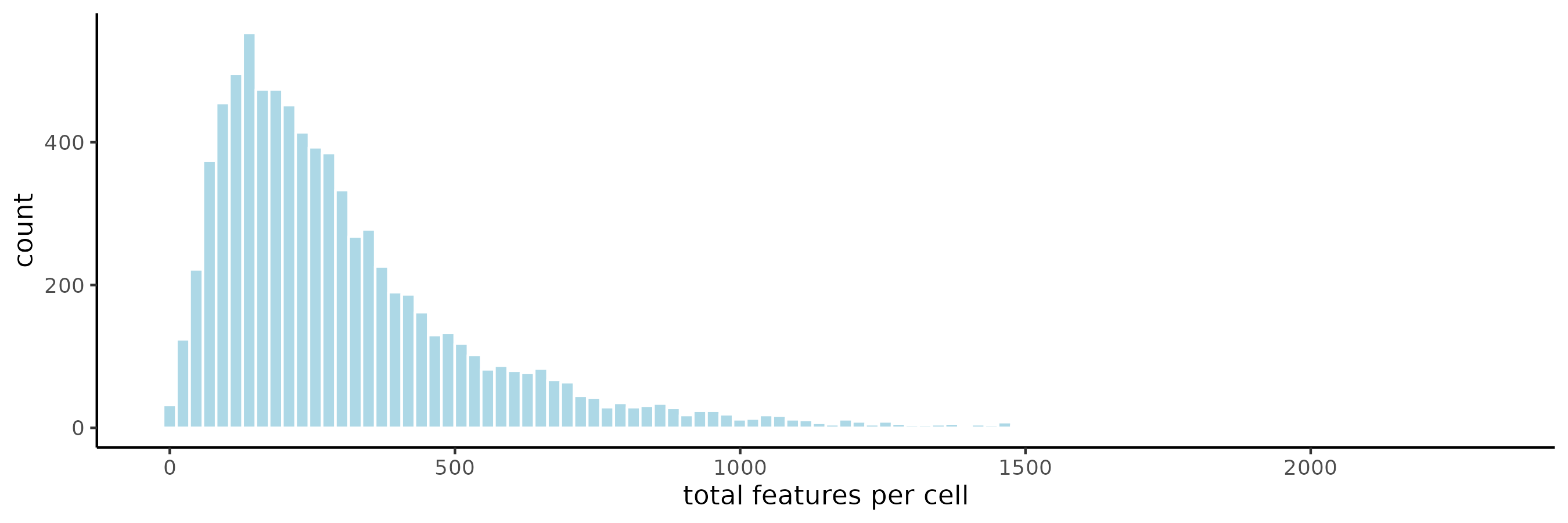
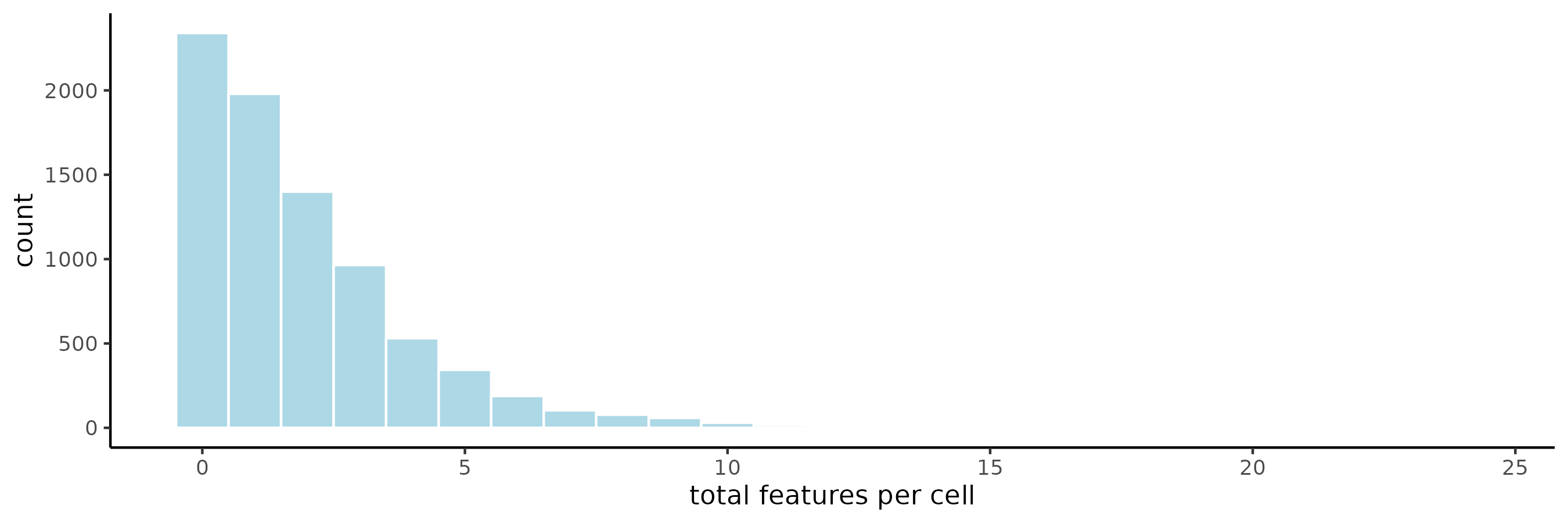
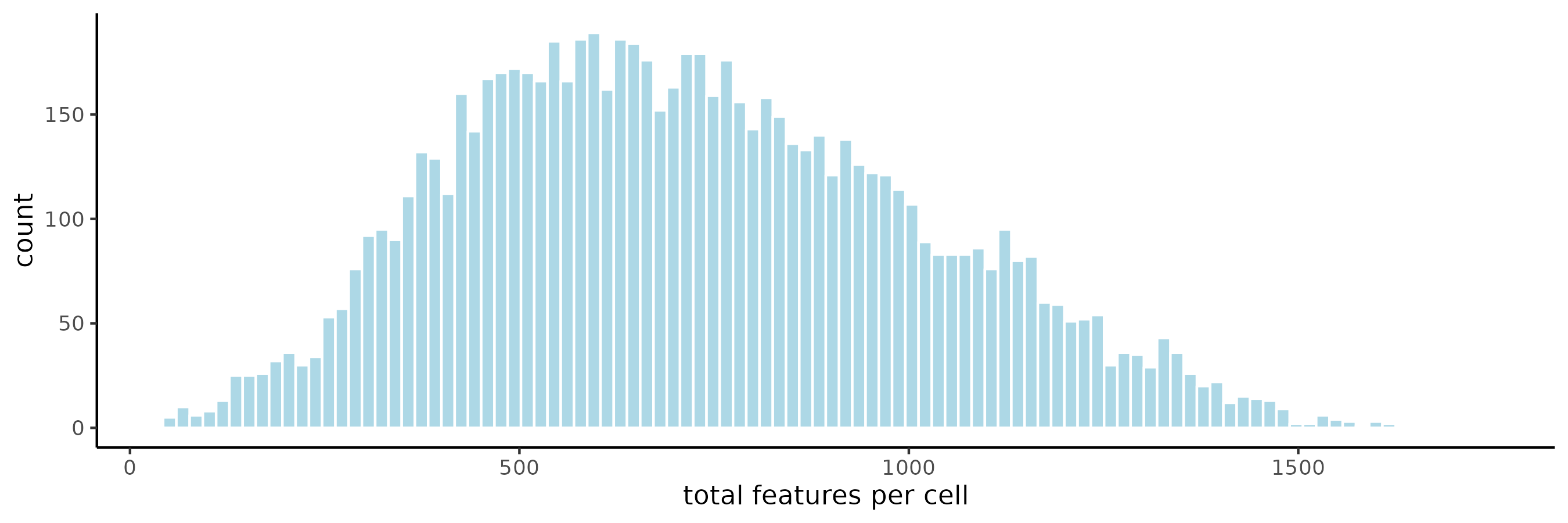
6.1 Plot histograms of total counts per cell#
filterDistributions(fov_join,
plot_type = 'hist',
detection = 'cells',
method = 'sum',
feat_type = 'rna',
nr_bins = 100,
save_param = list(base_height = 3,
save_name = '3.1_totalexpr'))
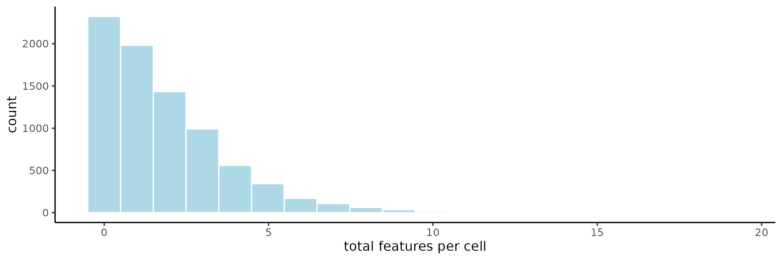
filterDistributions(fov_join,
plot_type = 'hist',
detection = 'cells',
method = 'sum',
feat_type = 'neg_probe',
nr_bins = 25,
save_param = list(base_height = 3,
save_name = '3.2_totalnegprbe'))
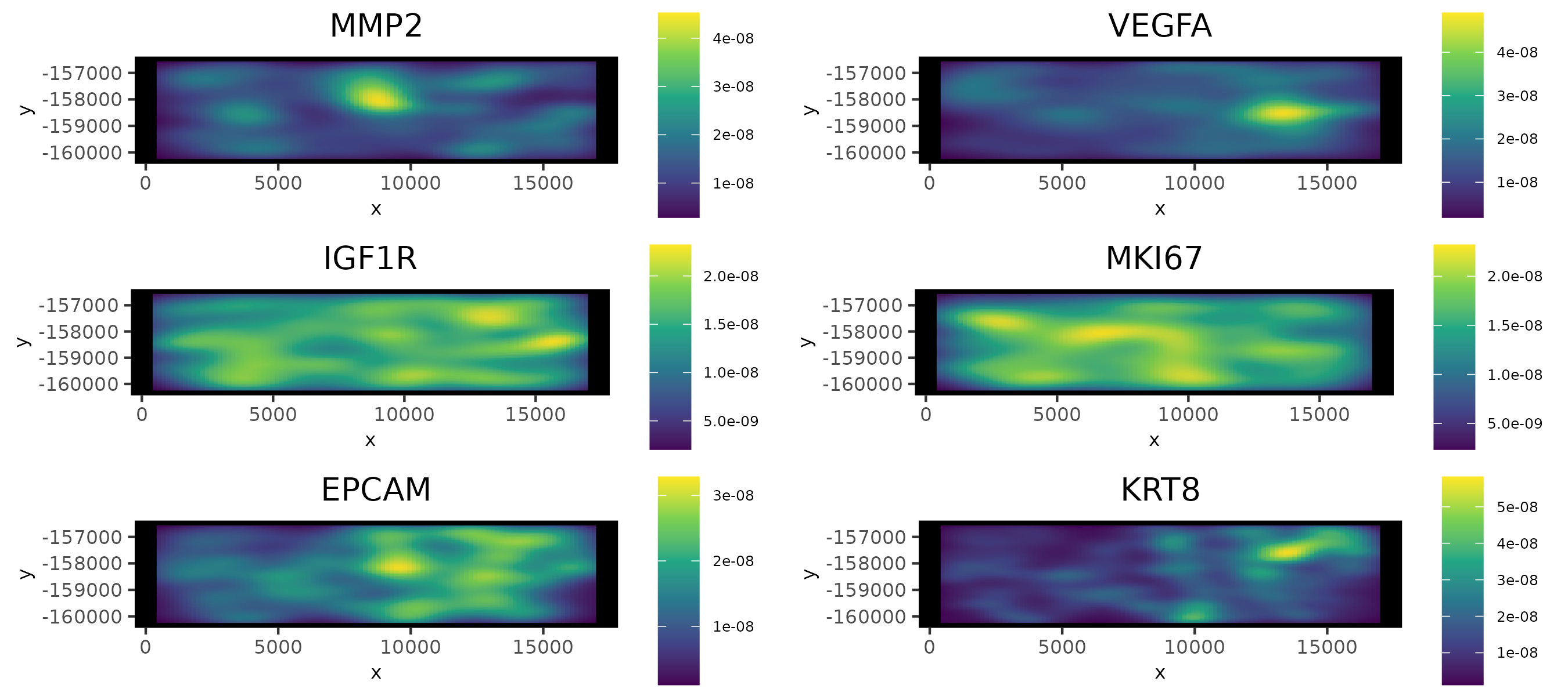
6.2 2D Density Plots#
Density-based representations may sometimes be preferred instead of
viewing the raw points information, especially when points are dense
enough that there is overplotting. After overlaps information has been
calculated, spatInSituPlotDensity() can be used in order to get a
general idea of how much expression there is of a feature.
spatInSituPlotDensity(gobject = fov_join,
                      feats = c("MMP2", "VEGFA", "IGF1R",
                                'MKI67', 'EPCAM', 'KRT8'),
                      cow_n_col = 2,
                      save_param = list(base_height = 4,
                                        save_name = '4_inSituDens'))
6.3 Extract Data from Giotto Object#
# combine cell data
morphometa = combineCellData(fov_join,
                             feat_type = 'rna')

# combine feature data
featmeta = combineFeatureData(fov_join,
                              feat_type = c('rna'))

# combine overlapping feature data
featoverlapmeta = combineFeatureOverlapData(fov_join,
                                            feat_type = c('rna'))
morphometa
# $rna
#                  cell_ID    sdimx     sdimy geom part          x         y hole list_ID feat
#       1:   fov002-cell_1  1025.82 -156627.0    1    1   979.4444 -156585.3    0  fov002  rna
#       2:   fov002-cell_1  1025.82 -156627.0    1    1  1043.4444 -156585.3    0  fov002  rna
#       3:   fov002-cell_1  1025.82 -156627.0    1    1  1043.4444 -156586.3    0  fov002  rna
#       4:   fov002-cell_1  1025.82 -156627.0    1    1  1048.4444 -156586.3    0  fov002  rna
#       5:   fov002-cell_1  1025.82 -156627.0    1    1  1048.4444 -156587.3    0  fov002  rna
#      ---
# 1280551: fov004-cell_999 15294.68 -158713.1 6378    1 15288.8889 -158685.3    0  fov004  rna
# 1280552: fov004-cell_999 15294.68 -158713.1 6378    1 15292.8889 -158685.3    0  fov004  rna
# 1280553: fov004-cell_999 15294.68 -158713.1 6378    1 15292.8889 -158683.3    0  fov004  rna
# 1280554: fov004-cell_999 15294.68 -158713.1 6378    1 15298.8889 -158683.3    0  fov004  rna
# 1280555: fov004-cell_999 15294.68 -158713.1 6378    1 15298.8889 -158681.3    0  fov004  rna
featmeta
# $rna
#          feat_ID    geom part         x         y hole z fov  CellComp   feat_ID_uniq feat spat_unit
#       1:    AATK   23962    1  3725.974 -160100.8    0 5   2  Membrane   fov002-23962  rna      cell
#       2:    AATK   28924    1  3344.687 -158576.3    0 5   2  Membrane   fov002-28924  rna      cell
#       3:    AATK   32363    1  4972.508 -158667.6    0 5   2         0   fov002-32363  rna      cell
#       4:    AATK   37076    1  4502.724 -158180.0    0 5   2         0   fov002-37076  rna      cell
#       5:    AATK   42621    1  2404.527 -158087.4    0 8   2         0   fov002-42621  rna      cell
#      ---
# 3331156:   ZFP36 3327938    1 16866.039 -160138.1    0 2   4   Nuclear fov004-1223368  rna      cell
# 3331157:   ZFP36 3328013    1 16842.374 -160133.1    0 1   4   Nuclear fov004-1223443  rna      cell
# 3331158:   ZFP36 3328281    1 16117.825 -160208.1    0 5   4 Cytoplasm fov004-1223711  rna      cell
# 3331159:   ZFP36 3328522    1 12781.322 -160146.5    0 2   4   Nuclear fov004-1223952  rna      cell
# 3331160:   ZFP36 3330762    1 16086.589 -160222.2    0 6   4   Nuclear fov004-1226192  rna      cell
featoverlapmeta
# $rna
#          feat_ID    geom part         x         y hole          poly_ID   feat_ID_uniq poly_info feat
#       1:    AATK   23962    1  3725.974 -160100.8    0             <NA>   fov002-23962      cell  rna
#       2:    AATK   28924    1  3344.687 -158576.3    0             <NA>   fov002-28924      cell  rna
#       3:    AATK   32363    1  4972.508 -158667.6    0 fov002-cell_1084   fov002-32363      cell  rna
#       4:    AATK   37076    1  4502.724 -158180.0    0             <NA>   fov002-37076      cell  rna
#       5:    AATK   42621    1  2404.527 -158087.4    0             <NA>   fov002-42621      cell  rna
#      ---
# 3331156:   ZFP36 3327938    1 16866.039 -160138.1    0 fov004-cell_2661 fov004-1223368      cell  rna
# 3331157:   ZFP36 3328013    1 16842.374 -160133.1    0 fov004-cell_2661 fov004-1223443      cell  rna
# 3331158:   ZFP36 3328281    1 16117.825 -160208.1    0 fov004-cell_2663 fov004-1223711      cell  rna
# 3331159:   ZFP36 3328522    1 12781.322 -160146.5    0 fov004-cell_2664 fov004-1223952      cell  rna
# 3331160:   ZFP36 3330762    1 16086.589 -160222.2    0 fov004-cell_2676 fov004-1226192      cell  rna
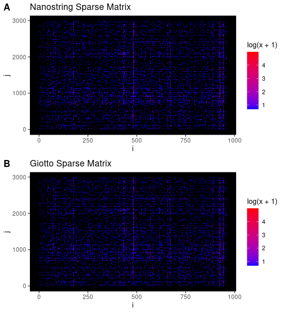
6.4 Comparison of Giotto aggregated and Nanostring provided matrices#
Comparison of Giotto’s aggregated matrix results and those provided by Nanostring. Only FOV2 will be used in this comparison. Matrices are expected to be similar when the same sets of cell polygons/masks are used for both.
# Load and prepare data

nanoDT = data.table::fread(paste0(data_path, 'Lung12_exprMat_file.csv'))
test1 = nanoDT[fov == 2]
# Set up cell_IDs
test1[, cell_ID := paste0('cell_', cell_ID)]
test1[, cell_ID := paste0('f', fov, '-', cell_ID)]
test1[, fov := NULL]

test1mat = Giotto:::t_flex(Giotto:::dt_to_matrix(test1))
testnano_f2 = test1mat
# Remove cell_0 (all tx counts that do not fall within a polygon)
testnano_f2 = testnano_f2[, -1]
# Remove negative probe counts
testnano_f2 = testnano_f2[!grepl('NegPrb', rownames(testnano_f2)),]

# giotto matrix
testg = fov_join@expression$cell$rna$raw[]
testg_f2 = testg[, grepl('fov002', colnames(testg))]
sorted_rownames = sort(rownames(testg_f2))
testg_f2 = testg_f2[sorted_rownames, ]

# Prepare matrix comparison
# Summarise sparse matrices (i and j are matrix indices, x is value)
testg_f2_DT = data.table::as.data.table(Matrix::summary(testg_f2))
testg_f2_DT[, method := 'giotto']
testnano_f2_DT = data.table::as.data.table(Matrix::summary(testnano_f2))
testnano_f2_DT[, method := 'nanostring']
testDT = data.table::rbindlist(list(testg_f2_DT, testnano_f2_DT))
# Combine sparse matrix indices
testDT[, combo := paste0(i,'-',j)]
# Plot results
library(ggplot2)

# matrix index similarity
pl_n = ggplot()
pl_n = pl_n + geom_tile(data = testnano_f2_DT, aes(x = i, y = j, fill = log(x+1)))
pl_n = pl_n + ggtitle('Nanostring Sparse Matrix')
pl_n = pl_n + scale_fill_gradient(low = 'blue', high = 'red')
pl_n = pl_n + theme(panel.grid.major = element_blank(),
                    panel.grid.minor = element_blank(),
                    panel.background = element_rect(fill = "black"))

pl_g = ggplot()
pl_g = pl_g + geom_tile(data = testg_f2_DT, aes(x = i, y = j, fill = log(x+1)))
pl_g = pl_g + ggtitle('Giotto Sparse Matrix')
pl_g = pl_g + scale_fill_gradient(low = 'blue', high = 'red')
pl_g = pl_g + theme(panel.grid.major = element_blank(),
                    panel.grid.minor = element_blank(),
                    panel.background = element_rect(fill = "black"))


combplot = cowplot::plot_grid(pl_n, pl_g,
                              nrow = 2,
                              labels = 'AUTO')
print(combplot)
# directly compare differences in matrix values (counts assigned)
vartestDT = testDT[, list(var = var(x), diff = diff(x), mean = mean(x)), by = .(i,j)]
data.table::setorder(vartestDT, var)

# check arbitrary index values
testDT[i == '812' & j == '2']
testDT[i == '667' & j == '1072']
testDT[i == '667' & j == '2880']

# plot difference in values
pl = ggplot()
pl = pl + geom_bar(data = vartestDT, aes(x = diff))
pl = pl + theme_bw()
pl = pl + labs(x = 'difference nanostring - Giotto')
pl

testDT[order(x)]
#      i j x method combo
# 1: 812 2 1 giotto 812-2
#
#      i    j  x     method    combo
# 1: 667 1072 50     giotto 667-1072
# 2: 667 1072 56 nanostring 667-1072
#
#      i    j  x     method    combo
# 1: 667 2880 24     giotto 667-2880
# 2: 667 2880 15 nanostring 667-2880
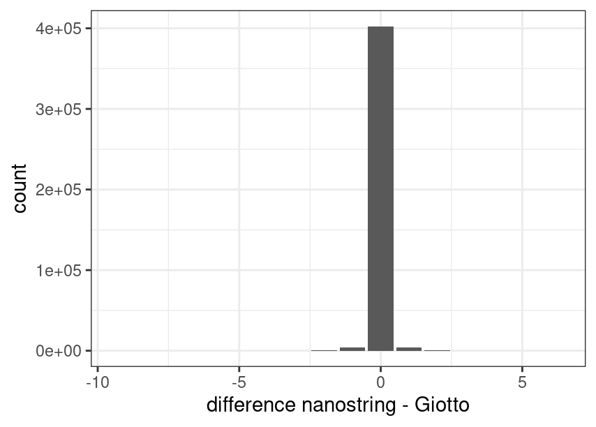
testDT[, .N, by = 'method']

testDT[, method, by = combo][, sum(duplicated(combo))]
#        method      N
# 1:     giotto 415952
# 2: nanostring 416099
#
# 411050
Overall, the nanostring matrix has 416099 - 415952 = 147 more non-zero values than giotto’s matrix for FOV2. Within the 411050 shared entries that were called by both methods (common i and j indices), there appears to be no major bias in terms of counts/values assigned. Moreover, the vast majority of these shared entries have the same values (difference of 0).
Back to convenience function: Section 1.1
7. Filtering and normalization#
standard normalization method: library size normalization and log normalization. This method will produce both normalized and scaled values that are be returned as the ‘normalized’ and ‘scaled’ expression matrices respectively. In this tutorial, the normalized values will be used for generating expression statistics and plotting expression values. The scaled values will be ignored. We will also generate normalized values for the negative probes for visualization purposes during which the library normalization step will be skipped.
pearson residuals: A normalization that uses the method described in Lause/Kobak et al. 2021. This produces a set of values that are most similar in utility to a scaled matrix and offer improvements to both HVF detection and PCA generation. These values should not be used for statistics, plotting of expression values, or differential expression analysis.
# filter (feat_type = 'rna' by default)
fov_join <- filterGiotto(gobject = fov_join,
                         feat_type = 'rna',
                         expression_threshold = 1,
                         feat_det_in_min_cells = 5,
                         min_det_feats_per_cell = 5)

# normalize
# standard method of normalization (log normalization based)
fov_join <- normalizeGiotto(gobject = fov_join,
                            feat_type = 'rna',
                            norm_methods = 'standard',
                            verbose = TRUE)
fov_join <- normalizeGiotto(gobject = fov_join,
                            feat_type = 'neg_probe',
                            norm_methods = 'standard',
                            library_size_norm = FALSE,
                            verbose = TRUE)

# new normalization method based on pearson correlations (Lause/Kobak et al. 2021)
# this normalized matrix is given the name 'pearson' using the update_slot param
fov_join <- normalizeGiotto(gobject = fov_join,
                            feat_type = 'rna',
                            scalefactor = 5000,
                            verbose = TRUE,
                            norm_methods = 'pearson_resid',
                            update_slot = 'pearson')

showGiottoExpression(fov_join)
expression
# └──Spatial unit "cell"
#    ├──Feature type "rna"
#    │  ├──Expression data "raw" values:
#    │  │     An object of class exprObj
#    │  │     for spatial unit: "cell" and feature type: "rna"
#    │  │       Provenance:  cell
#    │  │
#    │  │     contains:
#    │  │     960 x 8049 sparse Matrix of class "dgCMatrix"
#    │  │
#    │  │     LY6D  . . 1 . . . . . . . . . . ......
#    │  │     IGHA1 . . . . . . . 2 . 1 . . . ......
#    │  │     VWF   . . . 1 . . . . . 1 . . . ......
#    │  │
#    │  │      ........suppressing 8036 columns and 954 rows
#    │  │
#    │  │     CLEC2D 1 . . . . . . . . 1 . . . ......
#    │  │     MARCO  . . . . . . . . . . . . . ......
#    │  │     AATK   . . . . . . . . . . . . 2 ......
#    │  │
#    │  │      First four colnames:
#    │  │      fov002-cell_1 fov002-cell_2
#    │  │      fov002-cell_3 fov002-cell_4
#    │  │
#    │  ├──Expression data "normalized" values:
#    │  │     An object of class exprObj
#    │  │     for spatial unit: "cell" and feature type: "rna"
#    │  │       Provenance:  cell
#    │  │
#    │  │     contains:
#    │  │     960 x 8049 sparse Matrix of class "dgCMatrix"
#    │  │
#    │  │     LY6D  . . 4.666202 .        . . . .        . .       . . . ......
#    │  │     IGHA1 . . .        .        . . . 5.666544 . 4.70044 . . . ......
#    │  │     VWF   . . .        4.940306 . . . .        . 4.70044 . . . ......
#    │  │
#    │  │      ........suppressing 8036 columns and 954 rows
#    │  │
#    │  │     CLEC2D 4.146744 . . . . . . . . 4.70044 . . .        ......
#    │  │     MARCO  .        . . . . . . . . .       . . .        ......
#    │  │     AATK   .        . . . . . . . . .       . . 5.909612 ......
#    │  │
#    │  │      First four colnames:
#    │  │      fov002-cell_1 fov002-cell_2
#    │  │      fov002-cell_3 fov002-cell_4
#    │  │
#    │  ├──Expression data "scaled" values:
#    │  │     An object of class exprObj
#    │  │     for spatial unit: "cell" and feature type: "rna"
#    │  │       Provenance: cell
#    │  │
#    │  │     contains:
#    │  │     960 x 8049 dense matrix of class "dgeMatrix"
#    │  │
#    │  │                 [,1]        [,2]       [,3]       [,4]
#    │  │     LY6D  -0.4392934 -0.07558225  2.8787372 -0.3035845
#    │  │     IGHA1 -0.7570656 -0.51785331 -0.6631650 -0.6198371
#    │  │     VWF   -0.4387262 -0.07479291 -0.3300452  2.8316967
#    │  │     BECN1 -0.4359960 -0.07099306 -0.3271882 -0.3003029
#    │  │
#    │  │      First four colnames:
#    │  │      fov002-cell_1 fov002-cell_2
#    │  │      fov002-cell_3 fov002-cell_4
#    │  │
#    │  └──Expression data "pearson" values:
#    │        An object of class exprObj
#    │        for spatial unit: "cell" and feature type: "rna"
#    │          Provenance: cell
#    │
#    │        contains:
#    │        960 x 8049 dense matrix of class "dgeMatrix"
#    │
#    │                    [,1]       [,2]       [,3]       [,4]
#    │        LY6D  -0.4031565 -0.1363425  2.6585234 -0.3025217
#    │        IGHA1 -1.4462051 -0.4933275 -1.2011147 -1.0898172
#    │        VWF   -0.4178857 -0.1413313 -0.3460168  2.8722347
#    │        BECN1 -0.4074196 -0.1377863 -0.3373461 -0.3057230
#    │
#    │         First four colnames:
#    │         fov002-cell_1 fov002-cell_2
#    │         fov002-cell_3 fov002-cell_4
#    │
#    └──Feature type "neg_probe"
#       ├──Expression data "raw" values:
#       │     An object of class exprObj
#       │     for spatial unit: "cell" and feature type: "neg_probe"
#       │       Provenance:  cell
#       │
#       │     contains:
#       │     20 x 8049 sparse Matrix of class "dgCMatrix"
#       │
#       │     NegPrb8  . . . . . . . . . . 2 . . ......
#       │     NegPrb10 1 . . . . . . . . . . . 1 ......
#       │     NegPrb20 . . . . . . . . . . . . . ......
#       │
#       │      ........suppressing 8036 columns and 14 rows
#       │
#       │     NegPrb18 . . . . . . . . . . . . . ......
#       │     NegPrb12 . . . . . . . . . . . . . ......
#       │     NegPrb15 1 . 1 . . . . . . . . . . ......
#       │
#       │      First four colnames:
#       │      fov002-cell_1 fov002-cell_2
#       │      fov002-cell_3 fov002-cell_4
#       │
#       ├──Expression data "normalized" values:
#       │     An object of class exprObj
#       │     for spatial unit: "cell" and feature type: "neg_probe"
#       │       Provenance:  cell
#       │
#       │     contains:
#       │     20 x 8049 sparse Matrix of class "dgCMatrix"
#       │
#       │     NegPrb8  . . . . . . . . . . 1.584963 . . ......
#       │     NegPrb10 1 . . . . . . . . . .        . 1 ......
#       │     NegPrb20 . . . . . . . . . . .        . . ......
#       │
#       │      ........suppressing 8036 columns and 14 rows
#       │
#       │     NegPrb18 . . . . . . . . . . . . . ......
#       │     NegPrb12 . . . . . . . . . . . . . ......
#       │     NegPrb15 1 . 1 . . . . . . . . . . ......
#       │
#       │      First four colnames:
#       │      fov002-cell_1 fov002-cell_2
#       │      fov002-cell_3 fov002-cell_4
#       │
#       └──Expression data "scaled" values:
#             An object of class exprObj
#             for spatial unit: "cell" and feature type: "neg_probe"
#               Provenance: cell
#
#             contains:
#             20 x 8049 dense matrix of class "dgeMatrix"
#
#                            [,1]        [,2]       [,3]        [,4]
#             NegPrb8  -0.3207888  0.03413209 -0.4045849  0.03413209
#             NegPrb10  2.7851943  0.69791153 -0.3914547  0.69791153
#             NegPrb20 -0.3685845 -2.11549922 -0.4471068 -2.11549922
#             NegPrb21 -0.3472432 -1.15566687 -0.4281203 -1.15566687
#
#              First four colnames:
#              fov002-cell_1 fov002-cell_2
#              fov002-cell_3 fov002-cell_4
# add statistics based on log normalized values for features rna and negative probes
fov_join = addStatistics(gobject = fov_join,
                         expression_values = 'normalized',
                         feat_type = 'rna')
fov_join = addStatistics(gobject = fov_join,
                         expression_values = 'normalized',
                         feat_type = 'neg_probe')

# View cellular data (default is feat = 'rna')
showGiottoCellMetadata(fov_join)
# View feature data
showGiottoFeatMetadata(fov_join)
cell metadata
# └──Spatial unit "cell"
#    ├──Feature type "rna"
#    │     An object of class cellMetaObj
#    │     Provenance: cell
#    │              cell_ID list_ID nr_feats perc_feats total_expr
#    │     1: fov002-cell_1  fov002      203  21.145833   925.1119
#    │     2: fov002-cell_2  fov002       31   3.229167   231.4284
#    │     3: fov002-cell_3  fov002      140  14.583333   712.4315
#    │     4: fov002-cell_4  fov002      124  12.916667   652.3757
#    │
#    └──Feature type "neg_probe"
#          An object of class cellMetaObj
#          Provenance: cell
#                   cell_ID list_ID nr_feats perc_feats total_expr
#          1: fov002-cell_1  fov002        2         10          2
#          2: fov002-cell_2  fov002        0          0          0
#          3: fov002-cell_3  fov002        3         15          3
#          4: fov002-cell_4  fov002        0          0          0
feature metadata
# └──Spatial unit "cell"
#    ├──Feature type "rna"
#    │     An object of class featMetaObj
#    │     Provenance: cell
#    │        feat_ID nr_cells perc_cells total_expr mean_expr mean_expr_det
#    │     1:    LY6D      922   11.45484   3933.493 0.4886934      4.266262
#    │     2:   IGHA1     2900   36.02932  15960.468 1.9829131      5.503610
#    │     3:     VWF      919   11.41757   4047.916 0.5029092      4.404696
#    │     4:   BECN1      903   11.21878   3828.386 0.4756350      4.239630
#    │
#    └──Feature type "neg_probe"
#          An object of class featMetaObj
#          Provenance: cell
#              feat_ID nr_cells perc_cells total_expr  mean_expr mean_expr_det
#          1:  NegPrb8      642   7.976146   716.2937 0.08899164      1.115722
#          2: NegPrb10      566   7.031929   611.7775 0.07600664      1.080879
#          3: NegPrb20      888  11.032426  1003.0484 0.12461776      1.129559
#          4: NegPrb21      771   9.578830   849.4211 0.10553125      1.101713
Note: The show functions for metadata do not return the information.
To retrieve the metadata information, instead use pDataDT() and
fDataDT() along with the feat_type param for either ‘rna’ or
‘neg_probe’.
8. View Transcript Total Expression Distribution#
8.1 Histogram of log normalized data#
filterDistributions(fov_join,
                    detection = 'cells',
                    feat_type = 'rna',
                    expression_values = 'normalized',
                    method = 'sum',
                    nr_bins = 100,
                    save_param = list(base_height = 3,
                                      save_name = '5.1_rna_norm_total_hist'))

filterDistributions(fov_join,
                    detection = 'cell',
                    feat_type = 'neg_probe',
                    expression_values = 'normalized',
                    method = 'sum',
                    nr_bins = 20,
                    save_param = list(base_height = 3,
                                      save_name = '5.2_neg_norm_total_hist'))
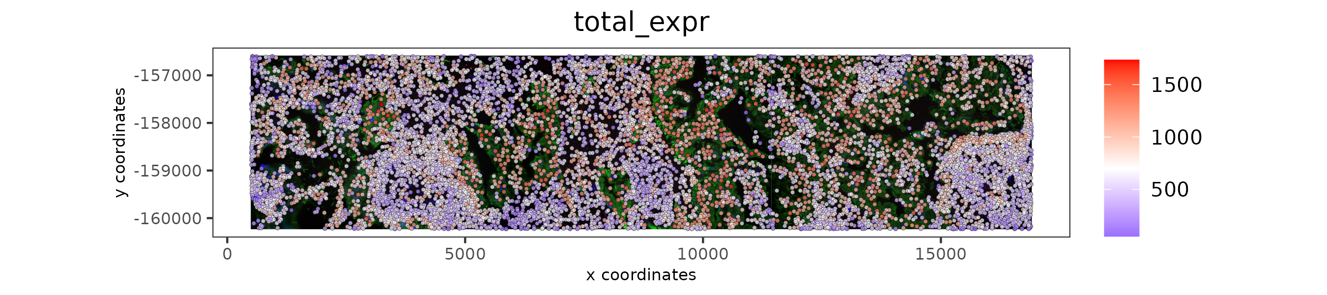
8.2 Plot spatially as centroids#
spatPlot2D(gobject = fov_join,
           cell_color = 'total_expr',
           color_as_factor = FALSE,
           show_image = TRUE,
           image_name = image_names,
           point_size = 0.9,
           point_alpha = 0.75,
           save_param = list(base_height = 2,
                             save_name = '5.3_color_centroids'))
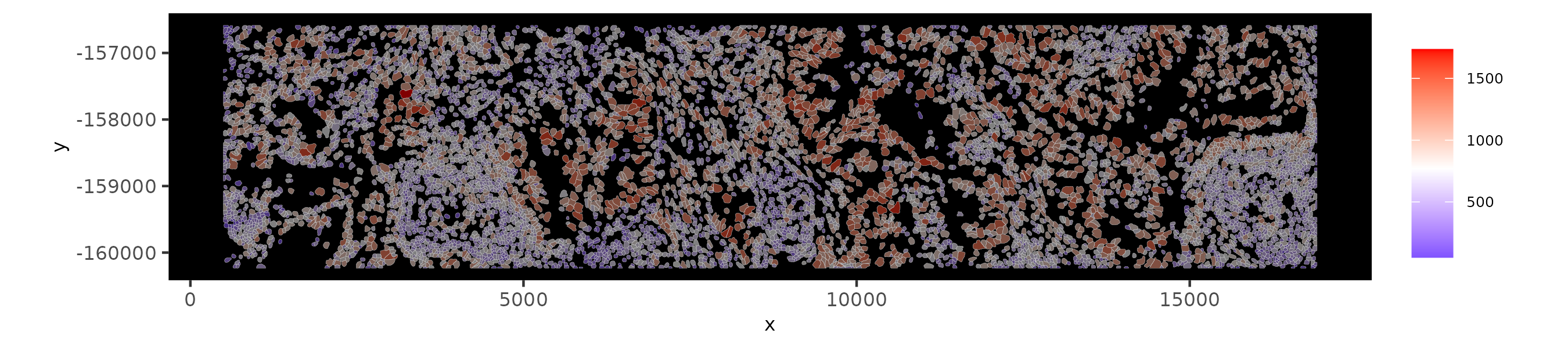
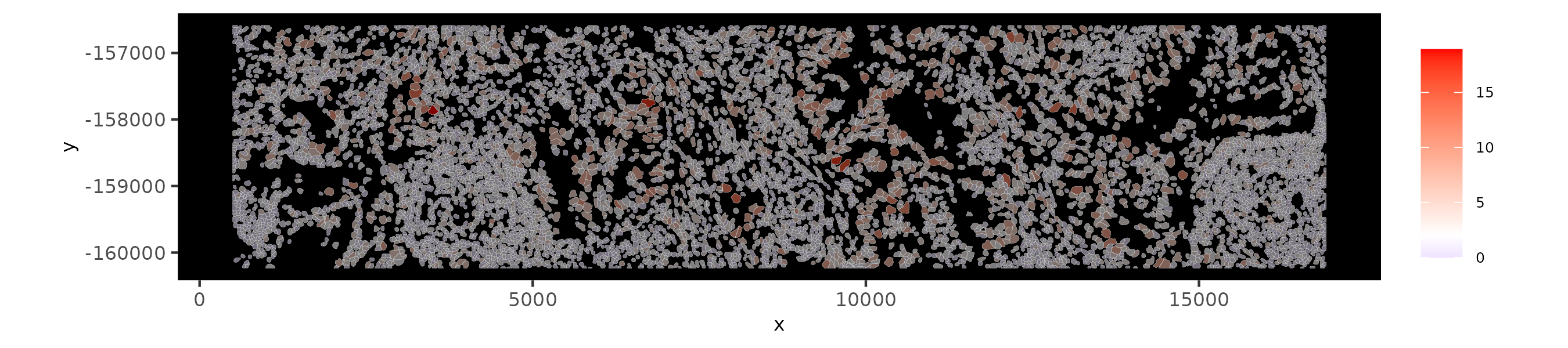
8.3 Plot spatially as color-scaled polygons#
spatInSituPlotPoints(fov_join,
                     show_polygon = TRUE,
                     polygon_color = 'gray',
                     polygon_line_size = 0.05,
                     polygon_fill = 'total_expr',
                     polygon_fill_as_factor = FALSE,
                     save_param = list(base_height = 2,
                                       save_name = '5.4_rna_color_polys'))

spatInSituPlotPoints(fov_join,
                     feat_type = 'neg_probe',
                     show_polygon = TRUE,
                     polygon_color = 'gray',
                     polygon_line_size = 0.05,
                     polygon_fill = 'total_expr',
                     polygon_fill_as_factor = FALSE,
                     save_param = list(base_height = 2,
                                       save_name = '5.5_neg_color_polys'))
9. Dimension Reduction#
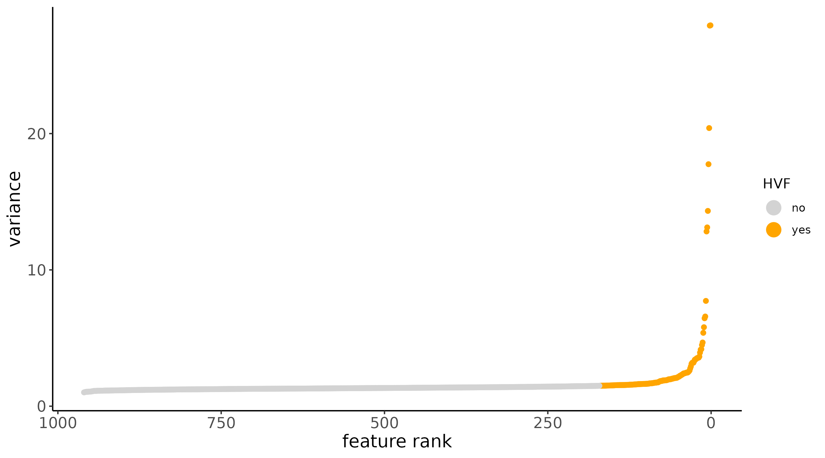
9.1 Detect highly variable genes and generate PCA#
fov_join = calculateHVF(fov_join,
                        method = 'var_p_resid',
                        expression_values = 'pearson',
                        save_param = list(base_height = 5,
                                          save_name = '6.1_pearson_HVF'))

# print HVFs
gene_meta = fDataDT(fov_join)
gene_meta[hvf == 'yes', feat_ID]
highly variable features
#   [1] "IGHA1"    "S100A4"   "NEAT1"    "MYH11"    "BMP6"
#   [6] "LGALS3"   "CLU"      "LTB"      "HLA-DQB1" "GDF15"
#  [11] "ENTPD1"   "CCL21"    "IL17A"    "GDNF"     "COL5A1"
#  [16] "HLA-B"    "IGKC"     "COL4A2"   "MZT2A"    "SERPINA1"
#  [21] "THBS1"    "MGP"      "IL32"     "HLA-DPA1" "RGS1"
#  [26] "IGFBP3"   "FCRLA"    "CXCL1"    "TYK2"     "KLF2"
#  [31] "HSPB1"    "ITGB6"    "COL6A1"   "WIF1"     "ANXA2"
#  [36] "THBS2"    "DUSP5"    "CXCL8"    "COL6A2"   "FGF2"
#  [41] "HSPA1A"   "TIMP1"    "TPM2"     "CD163"    "NPPC"
#  [46] "KRT8"     "IGHG1"    "CD68"     "SAA1"     "KRT7"
#  [51] "IGHM"     "IL1RN"    "B2M"      "LUM"      "FKBP11"
#  [56] "COL1A1"   "COL5A2"   "CX3CR1"   "MAF"      "TAGLN"
#  [61] "IL23A"    "BGN"      "FN1"      "DCN"      "CXCL10"
#  [66] "CD74"     "RARRES1"  "MALAT1"   "LTF"      "HLA-DRB5"
#  [71] "CALD1"    "C11orf96" "ADGRE2"   "MT1X"     "IGFBP5"
#  [76] "IGHG2"    "LCN2"     "TEK"      "PIGR"     "DUSP1"
#  [81] "IGFBP7"   "TM4SF1"   "DUSP2"    "CEACAM6"  "VIM"
#  [86] "FOS"      "COL9A2"   "CCL19"    "OLFM4"    "HLA-DPB1"
#  [91] "CXCL14"   "NFKBIA"   "HLA-DQA1" "CD14"     "HLA-C"
#  [96] "DLL1"     "KRT17"    "LDLR"     "CCL2"     "GLUL"
# [101] "TPSAB1"   "COL3A1"   "C1QA"     "S100A8"   "GSN"
# [106] "HSPA1B"   "MMP12"    "COL18A1"  "CIITA"    "HLA-DRB1"
# [111] "PSAP"     "SOD2"     "S100A2"   "LGALS1"   "STAT4"
# [116] "GADD45B"  "KDR"      "MMP14"    "KRT19"    "IL17D"
# [121] "MT2A"     "CXCR6"    "IL1B"     "FCGBP"    "CCL3L3"
# [126] "SPP1"     "CCL3"     "S100A6"   "IL16"     "ITGB4"
# [131] "RGCC"     "COL6A3"   "COL1A2"   "C1QC"     "CD8A"
# [136] "GZMK"     "TCL1A"    "IGF2"     "JCHAIN"   "SPARCL1"
# [141] "NDRG1"    "PSCA"     "CXCL3"    "HLA-DRA"  "CD79A"
# [146] "MEG3"     "SRGN"     "COL4A1"   "TNFRSF19" "ICAM1"
# [151] "RGS2"     "LYZ"      "CD83"     "CCL4L2"   "CD69"
# [156] "ACTA2"    "KRT5"     "MMP10"    "MMP2"     "CXCR5"
# [161] "CPA3"     "TPSB2"    "C1QB"     "CXCL2"    "CXCL5"
# [166] "AGR2"     "PDCD1"    "BCL2"     "XBP1"     "PDGFRB"
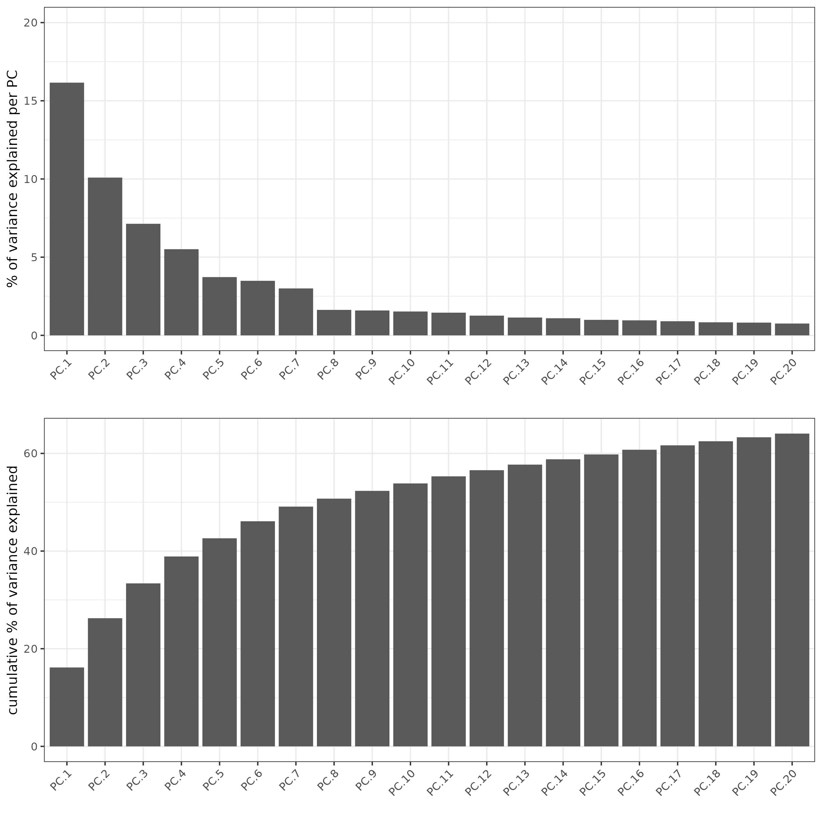
fov_join = runPCA(fov_join,
scale_unit = FALSE,
center = FALSE,
expression_values = 'pearson')
# screeplot uses the generated PCA. No need to specify expr values
screePlot(fov_join, ncp = 20, save_param = list(save_name = '6.2_screeplot'))
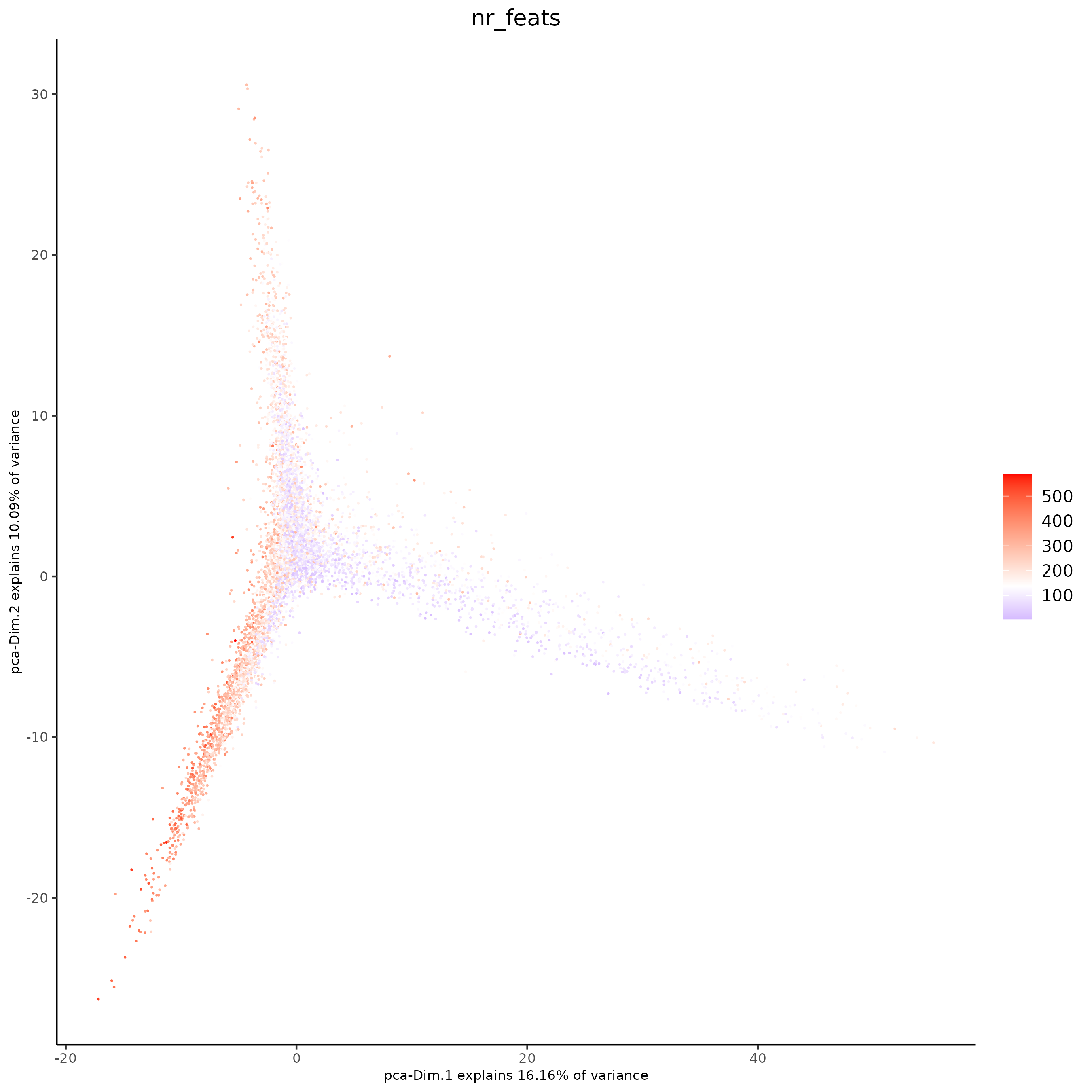
plotPCA(fov_join,
cell_color = 'nr_feats', # (from log norm statistics)
color_as_factor = FALSE,
point_size = 0.1,
point_shape = 'no_border',
save_param = list(save_name = '6.3_PCA'))
9.2 Run UMAP#
# Generate UMAP from PCA
fov_join <- runUMAP(fov_join,
dimensions_to_use = 1:10,
n_threads = 4)
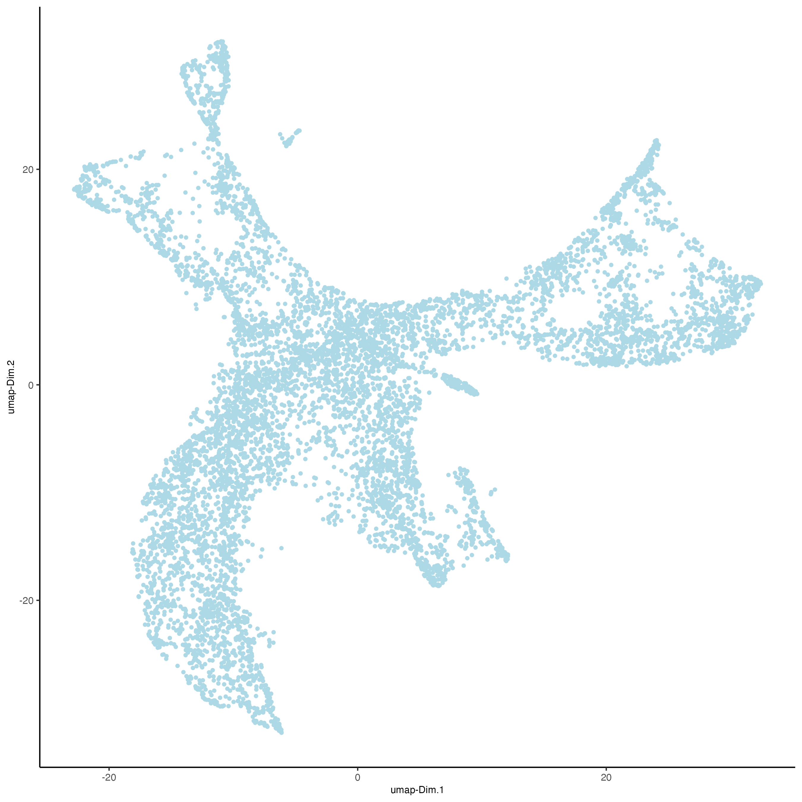
plotUMAP(gobject = fov_join, save_param = list(save_name = '6.4_UMAP'))
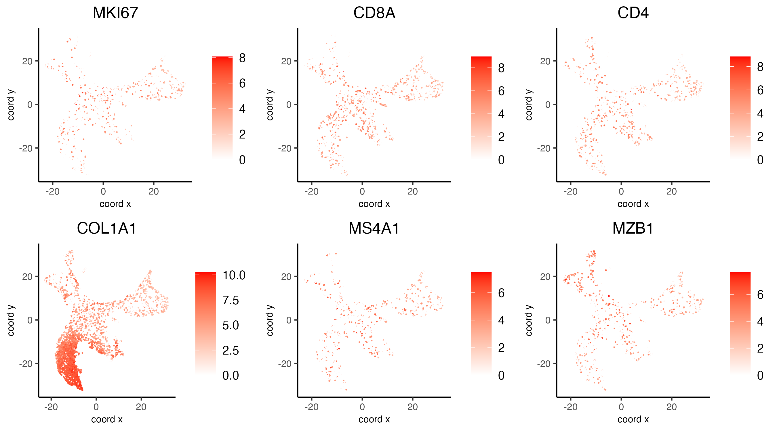
9.3 Plot features on expression space#
dimFeatPlot2D(gobject = fov_join,
              feat_type = 'rna',
              feats = c('MKI67', 'CD8A', 'CD4',
                        'COL1A1', 'MS4A1', 'MZB1'),
              expression_values = 'normalized',
              point_shape = 'no_border',
              point_size = 0.01,
              cow_n_col = 3,
              save_param = list(base_height = 5,
                                save_name = '6.5_UMAP_feats'))
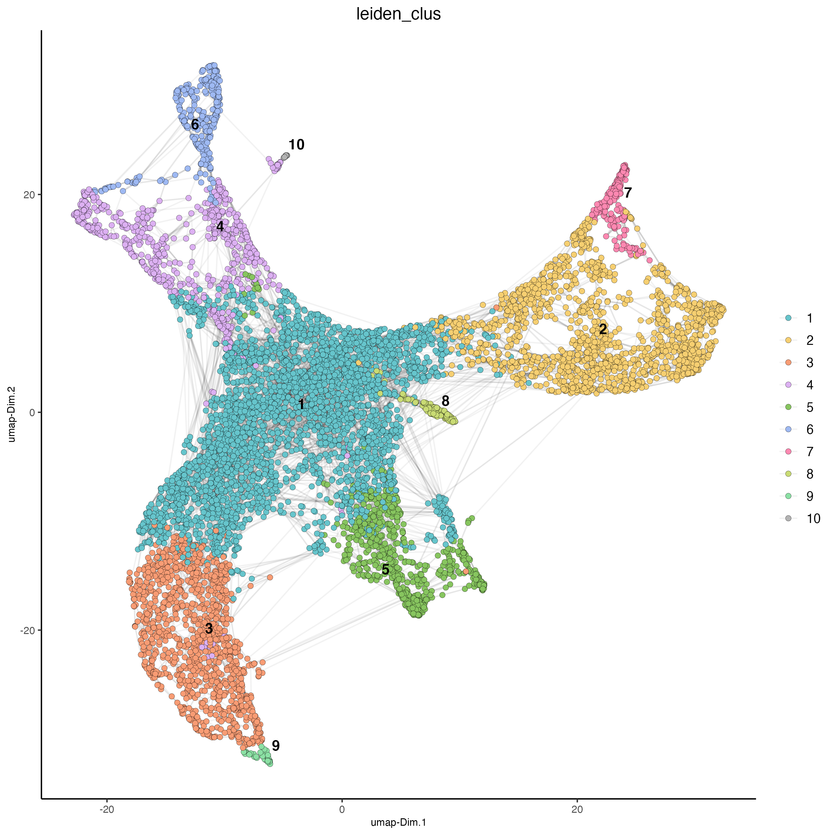
10. Cluster#
10.1 Visualize clustering#
fov_join <- createNearestNetwork(gobject = fov_join,
                                 dimensions_to_use = 1:10,
                                 k = 10)

fov_join <- doLeidenCluster(gobject = fov_join,
                            resolution = 0.07,
                            n_iterations = 1000)

# visualize UMAP cluster results
plotUMAP(gobject = fov_join,
         cell_color = 'leiden_clus',
         cell_color_code = pal10,
         show_NN_network = TRUE,
         point_size = 2,
         save_param = list(save_name = '7.1_UMAP_leiden'))
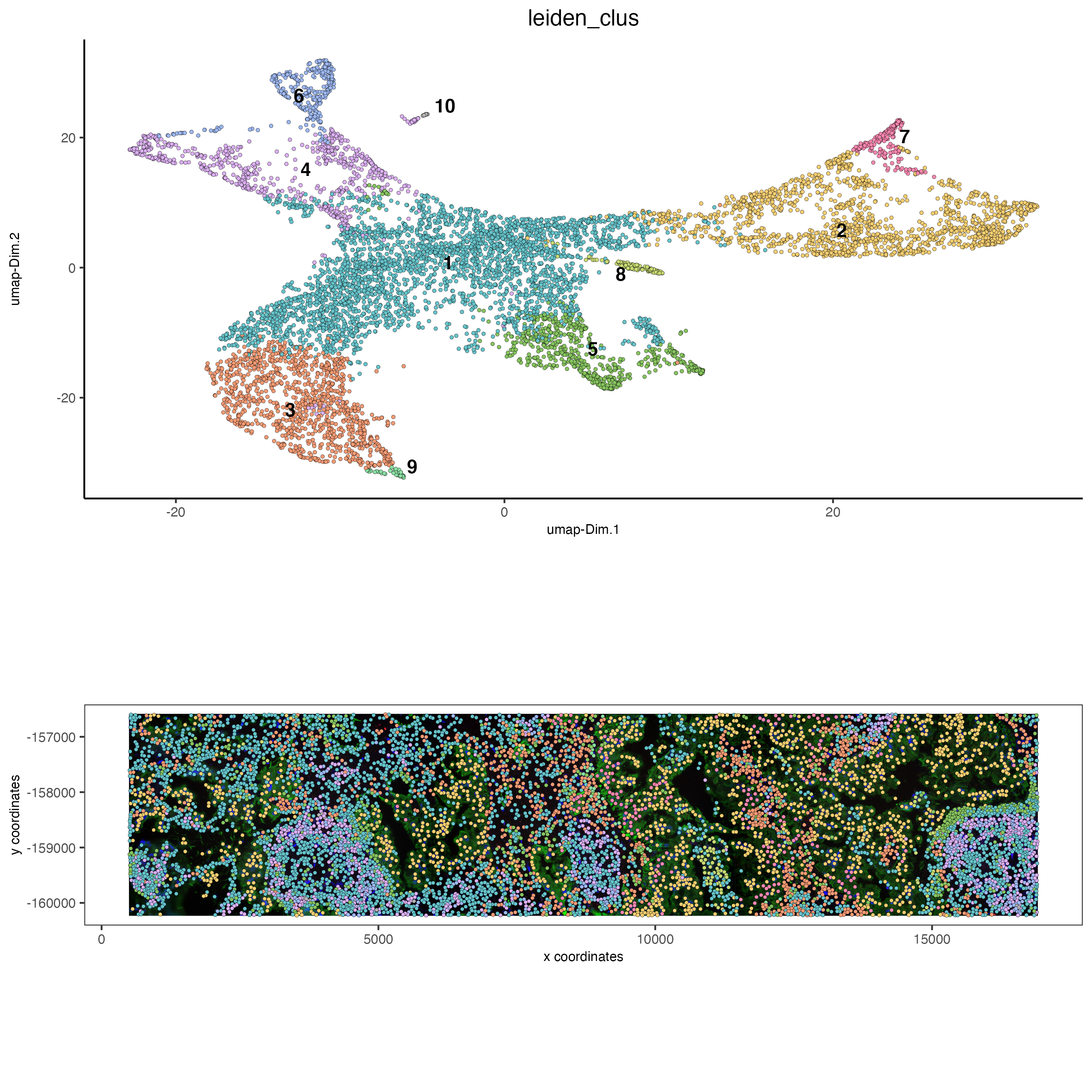
10.2 Visualize clustering on expression and spatial space#
# visualize UMAP and spatial results
spatDimPlot2D(gobject = fov_join,
              show_image = TRUE,
              image_name = image_names,
              cell_color = 'leiden_clus',
              cell_color_code = pal10,
              spat_point_size = 1,
              save_param = list(save_name = '7.2_spatdim_leiden'))
10.3 Map clustering spatially#
spatInSituPlotPoints(fov_join,
                     feats = list('rna' = c('MMP2', 'VEGFA', 'IGF1R',
                                            'MKI67', 'EPCAM', 'MZB1')),
                     point_size = 0.15,
                     feats_color_code = viv10,
                     show_polygon = TRUE,
                     polygon_color = 'white',
                     polygon_line_size = 0.01,
                     polygon_fill = 'leiden_clus',
                     polygon_fill_as_factor = TRUE,
                     polygon_fill_code = pal10,
                     save_param = list(base_height = 5,
                                       save_name = '7.3_spatinsitu_leiden'))
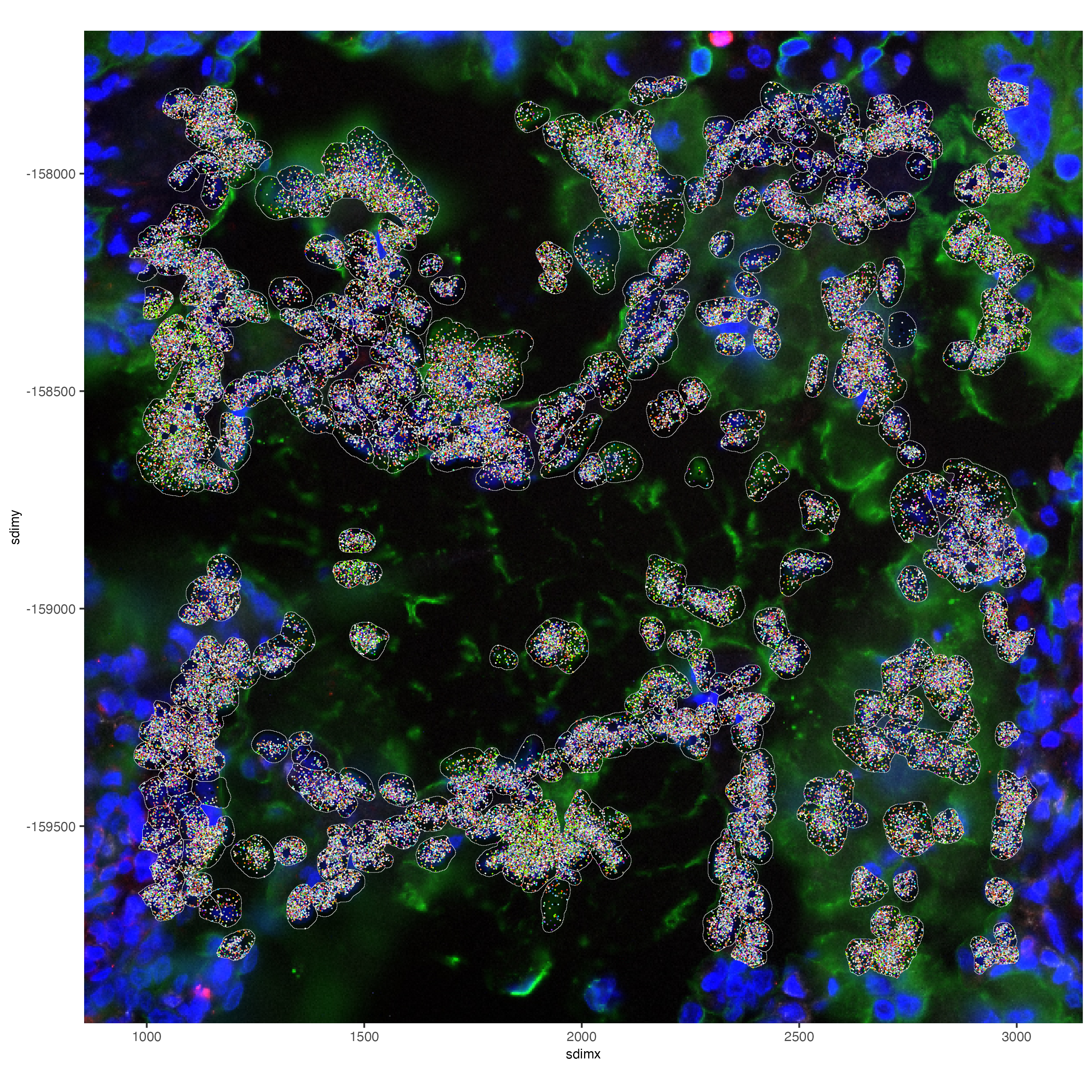
11. Small Subset Visualization#
#subset a Giotto object based on spatial locations
smallfov <- subsetGiottoLocs(fov_join,
x_max = 3000,
x_min = 1000,
y_max = -157800,
y_min = -159800)
#extract all genes observed in new object
smallfeats <- fDataDT(smallfov)[, feat_ID]
#plot all genes
spatInSituPlotPoints(smallfov,
feats = list(smallfeats),
point_size = 0.15,
polygon_line_size = 0.1,
show_polygon = TRUE,
polygon_color = 'white',
show_image = TRUE,
largeImage_name = 'fov002-composite',
show_legend = FALSE,
save_param = list(save_name = '8.1_smallfov_points'))
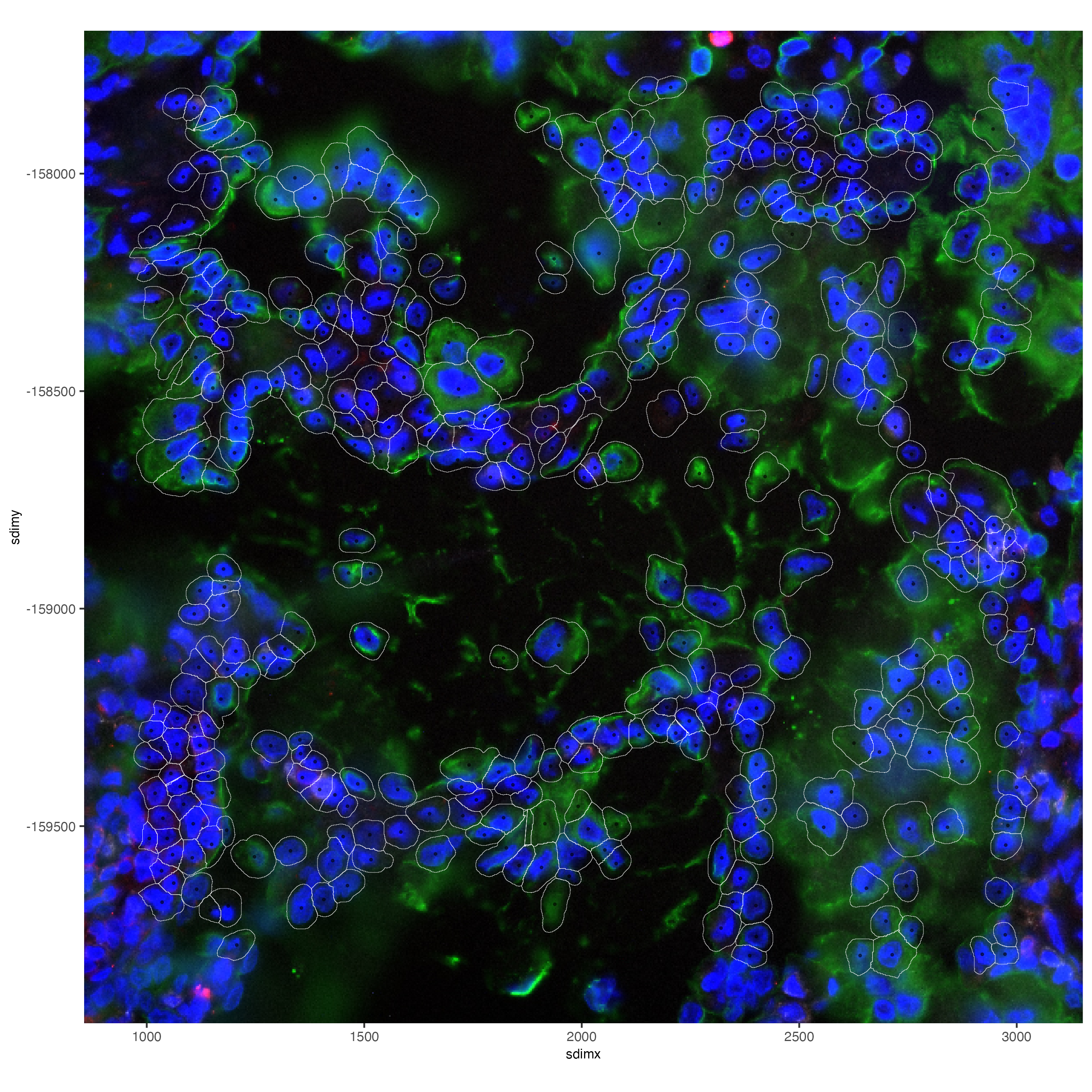
# plot only the polygon outlines
spatInSituPlotPoints(smallfov,
polygon_line_size = 0.1,
polygon_alpha = 0,
polygon_color = 'white',
show_polygon = TRUE,
show_image = TRUE,
largeImage_name = 'fov002-composite',
show_legend = FALSE,
save_param = list(save_name = '8.2_smallfov_poly'))
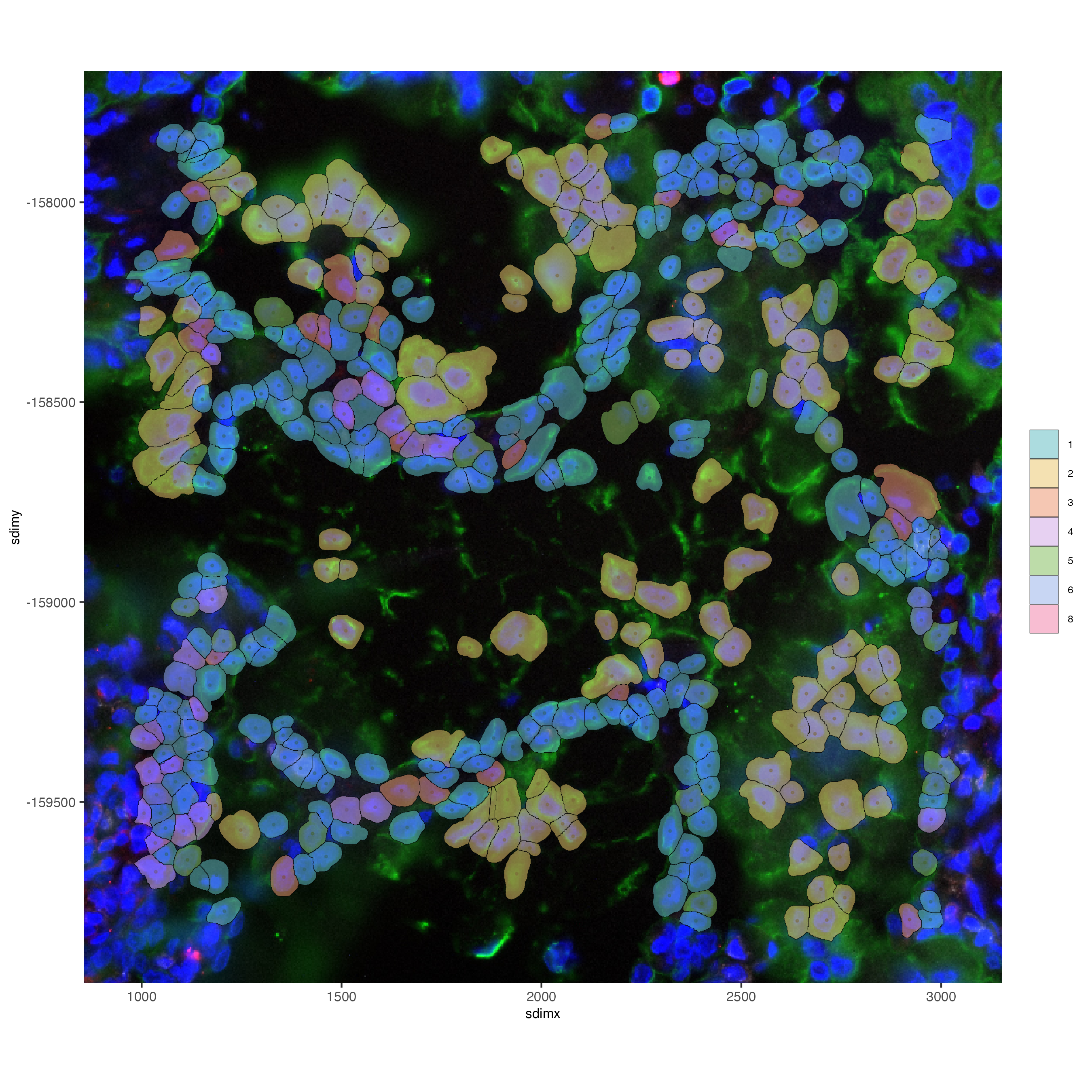
# plot polygons colorlabeled with leiden clusters
spatInSituPlotPoints(smallfov,
polygon_line_size = 0.1,
show_polygon = TRUE,
polygon_fill = 'leiden_clus',
polygon_fill_as_factor = TRUE,
polygon_fill_code = pal10,
show_image = TRUE,
largeImage_name = 'fov002-composite',
show_legend = FALSE,
save_param = list(save_name = '8.3_smallfov_leiden'))
12. Spatial Expression Patterns#
Find spatially organized gene expression by examining the binarized expression of cells and their spatial neighbors.
# create spatial network based on physical distance of cell centroids
fov_join = createSpatialNetwork(gobject = fov_join,
minimum_k = 2,
maximum_distance_delaunay = 50)
# perform Binary Spatial Extraction of genes - NOTE: Depending on your system this could take time
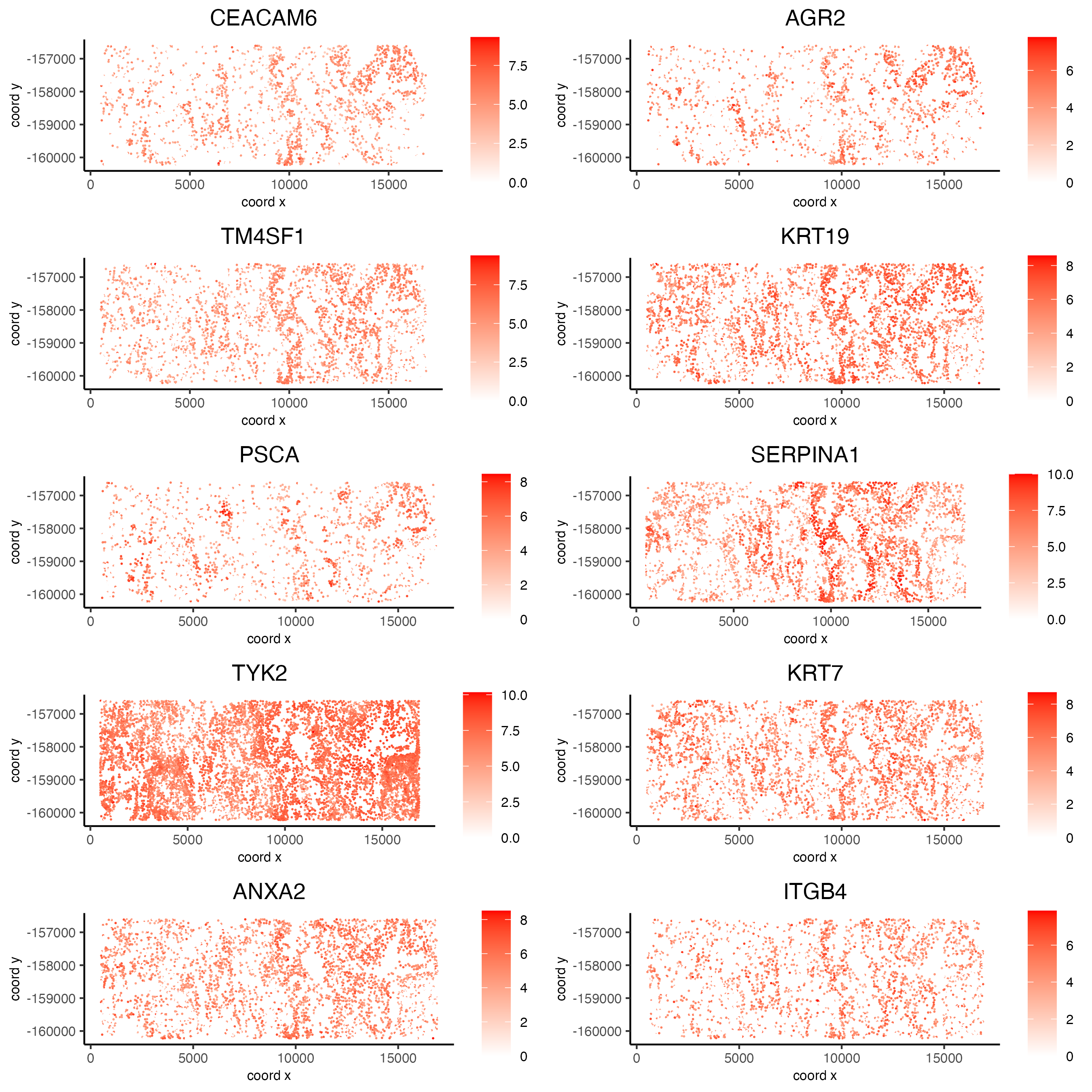
km_spatialgenes = binSpect(fov_join)
# visualize spatial expression of selected genes obtained from binSpect
spatFeatPlot2D(fov_join,
expression_values = 'normalized',
feats = km_spatialgenes$feats[1:10],
point_shape = 'no_border',
point_border_stroke = 0.01,
point_size = 0.01,
cow_n_col = 2,
save_param = list(save_name = '9_binspect_genes'))
13. Identify cluster differential expression genes#
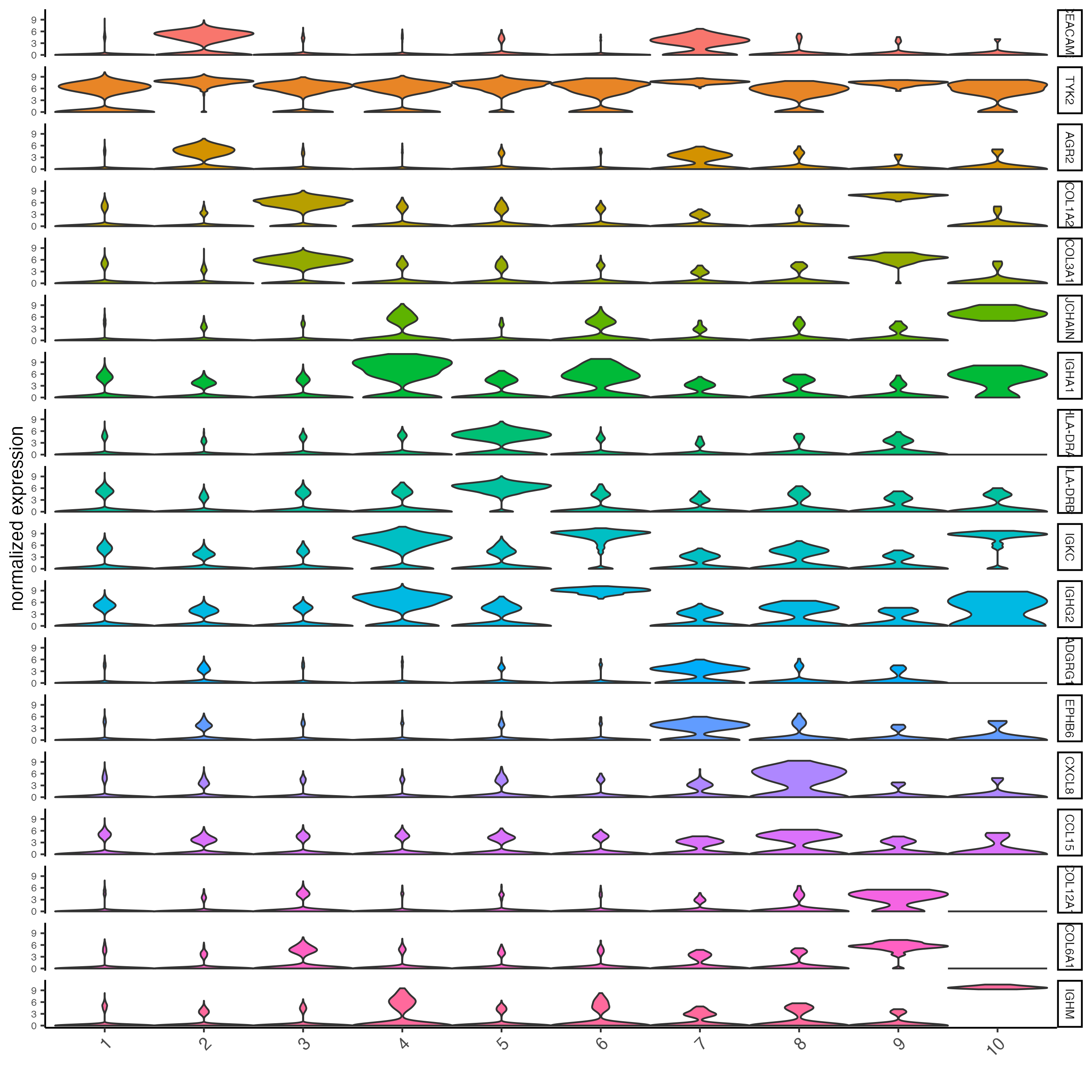
13.1 Violin plot#
# Gini
markers = findMarkers_one_vs_all(gobject = fov_join,
                                 method = 'gini',
                                 expression_values = 'normalized',
                                 cluster_column = 'leiden_clus',
                                 min_feats = 1,
                                 rank_score = 2)
# First 5 results by cluster
markers[, head(.SD, 5), by = 'cluster']

# violinplot
topgini_genes = unique(markers[, head(.SD, 2), by = 'cluster']$feats)
violinPlot(fov_join,
           feats = topgini_genes,
           cluster_column = 'leiden_clus',
           strip_position = 'right',
           save_param = list(save_name = '10.1_gini_violin'))
First 5 markers of each cluster
#     cluster    feats expression expression_gini  detection detection_gini expression_rank detection_rank   comb_score comb_rank
#  1:       1  CEACAM6  0.3005461      0.32848944 0.06234867     0.32595794             0.1           0.55 5.889056e-03         1
#  2:       1     TYK2  4.3646431      0.08881957 0.67493947     0.07004094             0.1           0.55 3.421554e-04       457
#  3:       1    RAMP1  2.8381932      0.04598805 0.50665860     0.07329526             0.1           0.55 1.853888e-04       696
#  4:       1   COL9A2  3.3775202      0.02803581 0.58353511     0.05483438             0.1           0.55 8.455294e-05       857
#  5:       1     WIF1  3.6318024      0.02295722 0.62046005     0.04942676             0.1           0.55 6.240854e-05       885
#  6:       2  CEACAM6  3.5574984      0.40305510 0.69286658     0.38975970             1.0           1.00 1.570946e-01         1
#  7:       2     AGR2  2.8990604      0.39072866 0.60237781     0.38035439             1.0           1.00 1.486154e-01         2
#  8:       2     PSCA  2.7500933      0.37081552 0.54821664     0.35942508             1.0           1.00 1.332804e-01         3
#  9:       2   TM4SF1  4.2980932      0.34496868 0.80581242     0.33059895             1.0           1.00 1.140463e-01         4
# 10:       2    ITGB4  2.9779267      0.31322641 0.64266843     0.31854817             1.0           1.00 9.977770e-02         5
# 11:       3   COL1A2  5.1763307      0.35868057 0.84092940     0.32712715             1.0           1.00 1.173342e-01         1
# 12:       3   COL3A1  4.6626627      0.35227376 0.79624665     0.32419688             1.0           1.00 1.142061e-01         2
# 13:       3   COL5A1  2.8124393      0.30790277 0.54870420     0.29029496             1.0           1.00 8.938262e-02         6
# 14:       3    CALD1  2.7964416      0.29034672 0.53976765     0.27132087             1.0           1.00 7.877712e-02         7
# 15:       3   COL4A2  3.7519663      0.28290733 0.66041108     0.25489261             1.0           1.00 7.211099e-02         8
# 16:       4   JCHAIN  2.3085145      0.31920894 0.38356164     0.27096015             1.0           1.00 8.649290e-02         1
# 17:       4    IGHA1  6.0272393      0.29235201 0.77123288     0.20720352             1.0           1.00 6.057637e-02         2
# 18:       4     IGKC  6.0069266      0.27710427 0.80821918     0.21309249             1.0           1.00 5.904884e-02         3
# 19:       4    IGHG2  5.1049710      0.21301372 0.75753425     0.16159106             1.0           1.00 3.442111e-02         5
# 20:       4    IGHG1  6.0348289      0.21398818 0.84109589     0.15579987             1.0           1.00 3.333933e-02         6
# 21:       5  HLA-DRA  3.5278230      0.35261913 0.68000000     0.33461396             1.0           1.00 1.179913e-01         1
# 22:       5 HLA-DRB1  5.8080578      0.31796037 0.94000000     0.28322219             1.0           1.00 9.005343e-02         4
# 23:       5     C1QC  2.9167826      0.30428046 0.56153846     0.28012788             1.0           1.00 8.523744e-02         5
# 24:       5 HLA-DQA1  3.4158034      0.29287085 0.66307692     0.27394289             1.0           1.00 8.022989e-02         7
# 25:       5 HLA-DPA1  4.5054688      0.29433678 0.81076923     0.26644593             1.0           1.00 7.842484e-02         8
# 26:       6     IGKC  7.7995871      0.30816788 0.91193182     0.22600725             1.0           1.00 6.964818e-02         1
# 27:       6    IGHG2  8.9434075      0.31508193 1.00000000     0.21706726             1.0           1.00 6.839397e-02         3
# 28:       6     XBP1  3.0542933      0.25791147 0.55681818     0.21972330             1.0           1.00 5.666916e-02         4
# 29:       6    IGHG1  9.6683517      0.29921666 1.00000000     0.18784629             1.0           1.00 5.620674e-02         5
# 30:       6    IGHA1  3.9283810      0.17471016 0.61931818     0.13994645             1.0           1.00 2.445007e-02         9
# 31:       7   ADGRG1  2.3821747      0.34229952 0.62827225     0.35696837             1.0           1.00 1.221901e-01         1
# 32:       7    EPHB6  2.6829243      0.33650319 0.68586387     0.34987822             1.0           1.00 1.177351e-01         2
# 33:       7   SLC2A1  2.7642290      0.31840437 0.70680628     0.33418653             1.0           1.00 1.064065e-01         3
# 34:       7   S100A2  5.2415295      0.33596555 0.92670157     0.31263296             1.0           1.00 1.050339e-01         4
# 35:       7    ITGA3  4.2001159      0.32268560 0.91099476     0.31732234             1.0           1.00 1.023953e-01         5
# 36:       8    CXCL8  3.8332176      0.34293929 0.62500000     0.30076350             1.0           1.00 1.031436e-01         1
# 37:       8    CCL15  2.5480321      0.17891558 0.52500000     0.16468271             1.0           1.00 2.946430e-02        51
# 38:       8    KRT18  2.5900116      0.11144915 0.54166667     0.10688863             1.0           1.00 1.191265e-02       225
# 39:       8     RARA  3.0165397      0.10350445 0.61666667     0.09770431             1.0           1.00 1.011283e-02       269
# 40:       8    RPL21  3.8977863      0.09196966 0.74166667     0.08031020             1.0           1.00 7.386102e-03       335
# 41:       9  COL12A1  3.1357798      0.37144461 0.74000000     0.37663390             1.0           1.00 1.398986e-01         1
# 42:       9   COL6A1  5.4311138      0.37885115 0.96000000     0.35502793             1.0           1.00 1.345027e-01         2
# 43:       9   COL6A3  5.3010486      0.37021296 0.96000000     0.35369715             1.0           1.00 1.309433e-01         3
# 44:       9      LUM  4.1146700      0.36697530 0.82000000     0.35593448             1.0           1.00 1.306192e-01         4
# 45:       9   COL6A2  5.5736044      0.36936888 1.00000000     0.34879032             1.0           1.00 1.288323e-01         5
# 46:      10   JCHAIN  6.9947297      0.41405696 1.00000000     0.38000000             1.0           1.00 1.573416e-01         1
# 47:      10     IGHM  9.7929156      0.41818020 1.00000000     0.34508525             1.0           1.00 1.443078e-01         2
# 48:      10     IGKC  7.5834742      0.28325352 0.89473684     0.20871211             1.0           1.00 5.911844e-02         4
# 49:      10    IGHA1  4.4631436      0.19301447 0.73684211     0.17215134             1.0           1.00 3.322770e-02        18
# 50:      10    IGHG1  5.1429134      0.15242469 0.84210526     0.13847022             1.0           1.00 2.110628e-02        40
#     cluster    feats expression expression_gini  detection detection_gini expression_rank detection_rank   comb_score comb_rank
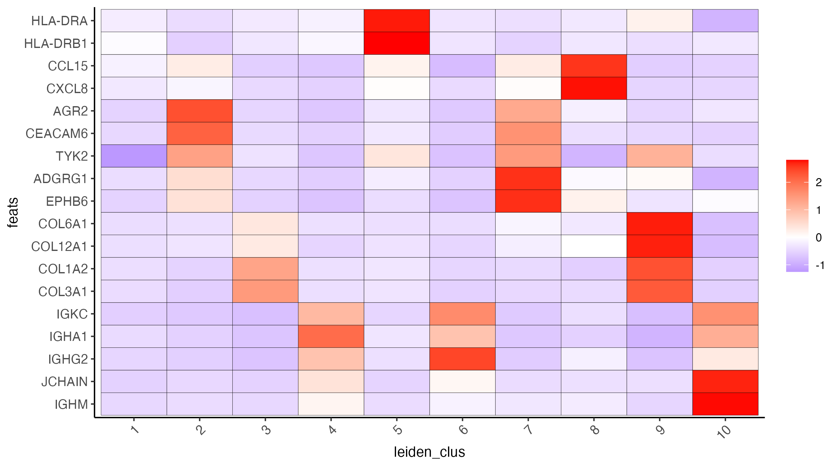
13.2 Heatmap#
cluster_order = 1:10
plotMetaDataHeatmap(fov_join,
                    expression_values = 'normalized',
                    metadata_cols = c('leiden_clus'),
                    selected_feats = topgini_genes,
                    custom_cluster_order = cluster_order,
                    save_param = list(base_height = 5,
                                      save_name = '10.2_heatmap'))
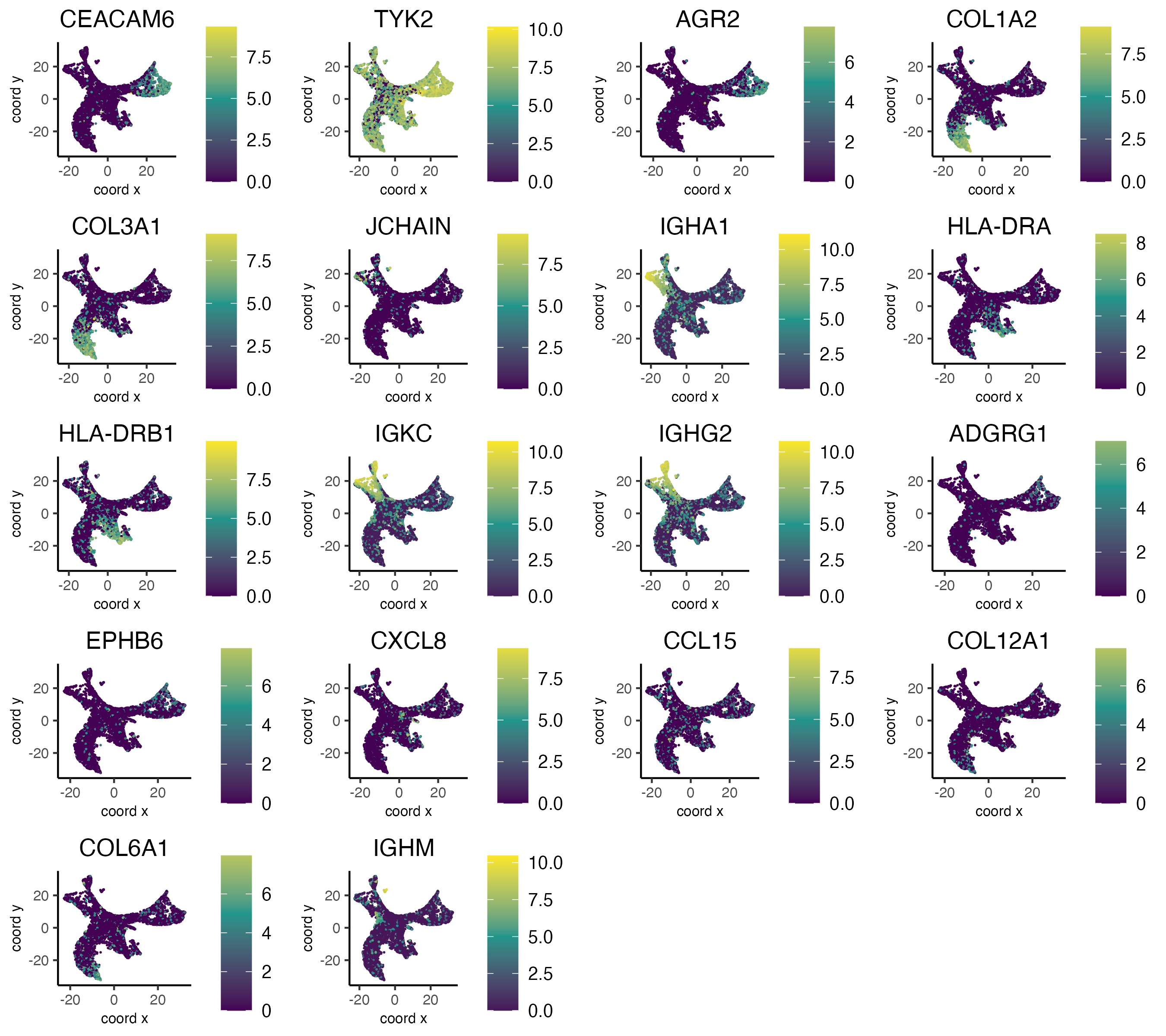
13.3 Plot gini genes on UMAP#
# low, mid, high
custom_scale = c('#440154', '#1F968B', '#FDE725')

dimFeatPlot2D(fov_join,
              expression_values = 'normalized',
              cell_color_gradient = custom_scale,
              gradient_midpoint = 5,
              feats = topgini_genes,
              point_shape = 'no_border',
              point_size = 0.001,
              cow_n_col = 4,
              save_param = list(base_height = 8,
                                save_name = '10.3_gini_genes'))
13.4 Annotate Giotto Object#
## add cell types ###
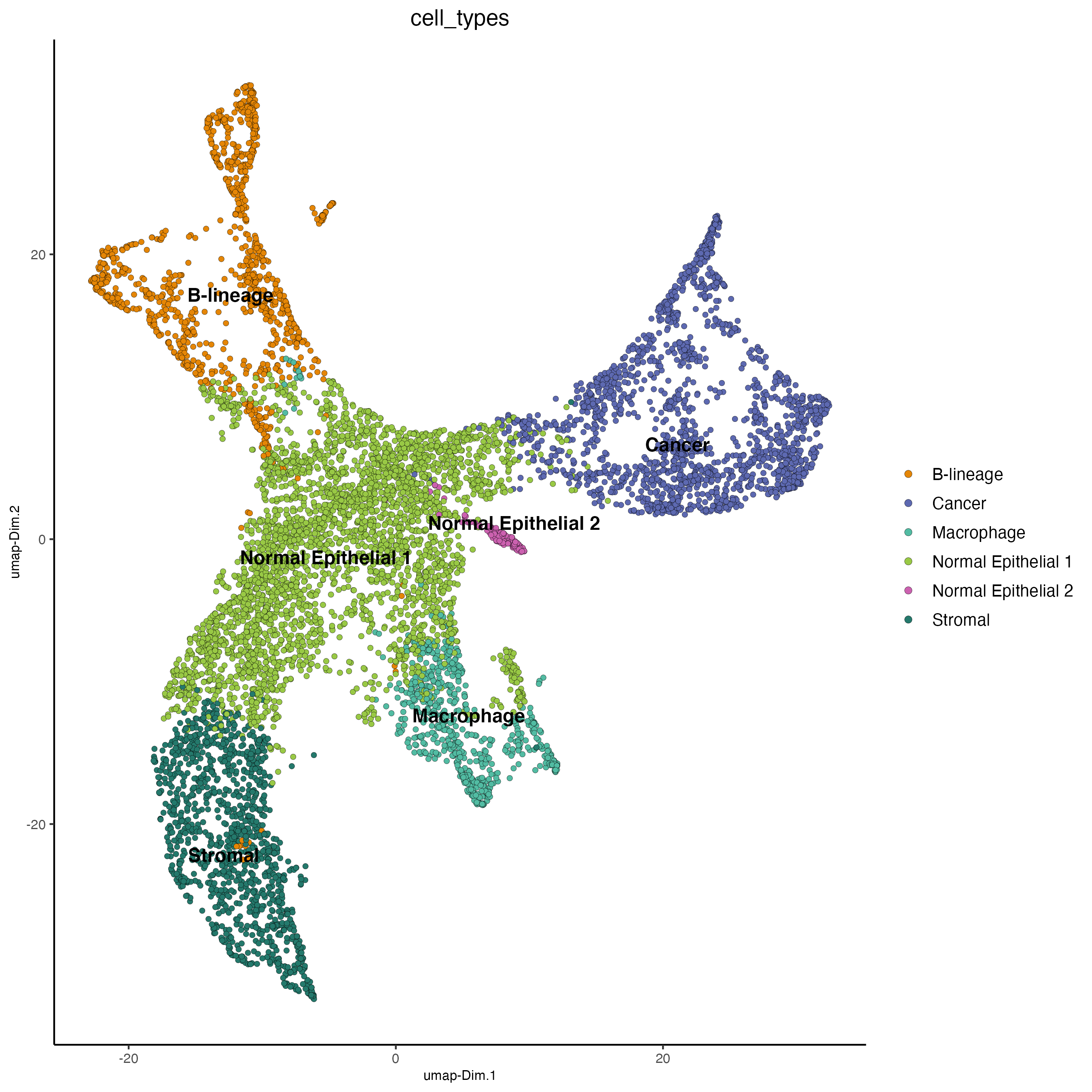
clusters_cell_types_lung = c('Normal Epithelial 1', 'Cancer', 'Stromal', 'B-lineage',
'Macrophage', 'B-lineage', 'Cancer',
'Normal Epithelial 2', 'Stromal', 'B-lineage')
names(clusters_cell_types_lung) = 1:10
fov_join = annotateGiotto(gobject = fov_join,
annotation_vector = clusters_cell_types_lung,
cluster_column = 'leiden_clus',
name = 'cell_types')
plotUMAP(fov_join,
cell_color = 'cell_types',
cell_color_code = viv10,
point_size = 1.5,
save_param = list(save_name = '11_anno_umap'))
13.5 Visualize#
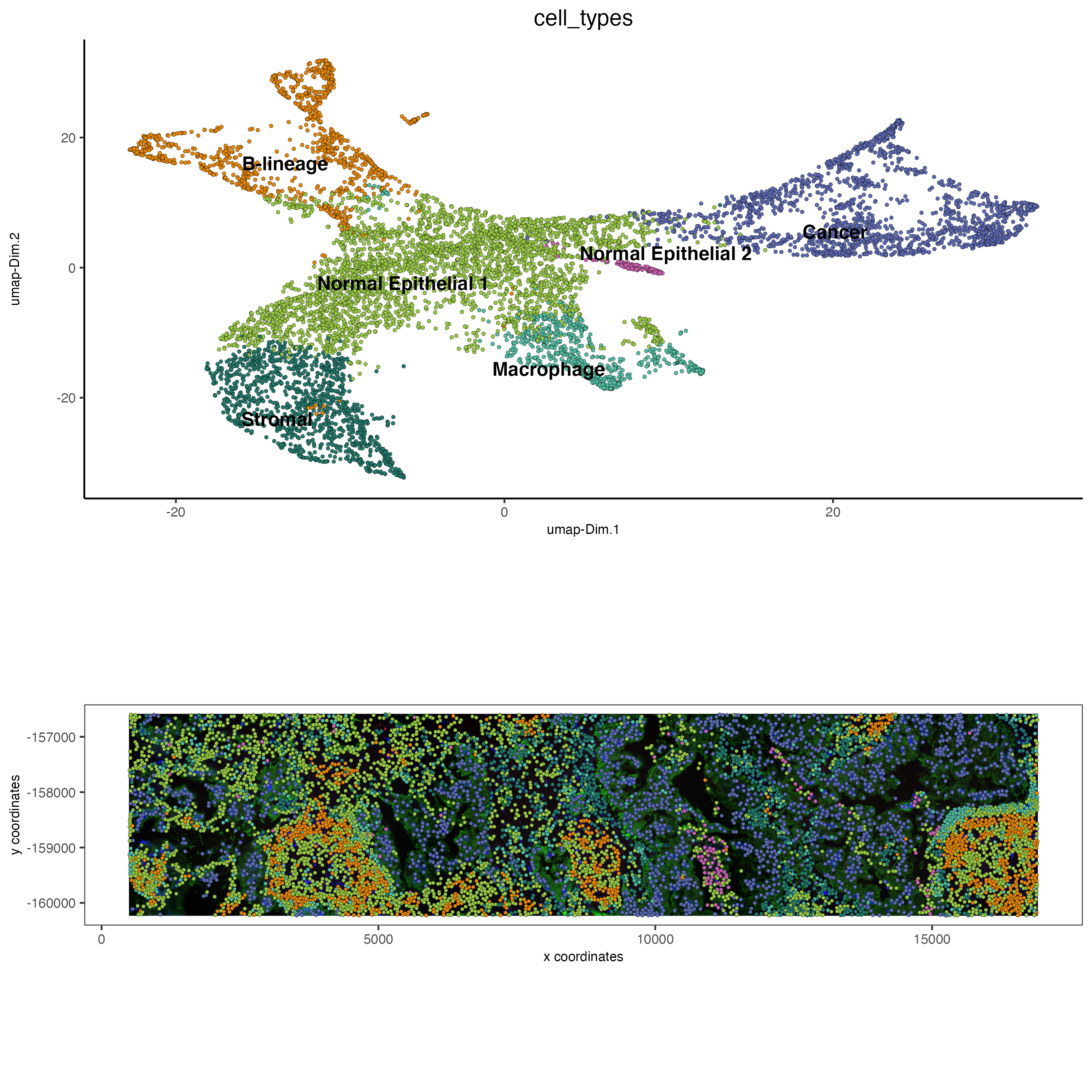
spatDimPlot2D(gobject = fov_join,
              show_image = TRUE,
              image_name = image_names,
              cell_color = 'cell_types',
              cell_color_code = viv10,
              spat_point_size = 1,
              save_param = list(save_name = '12_spatdim_type'))
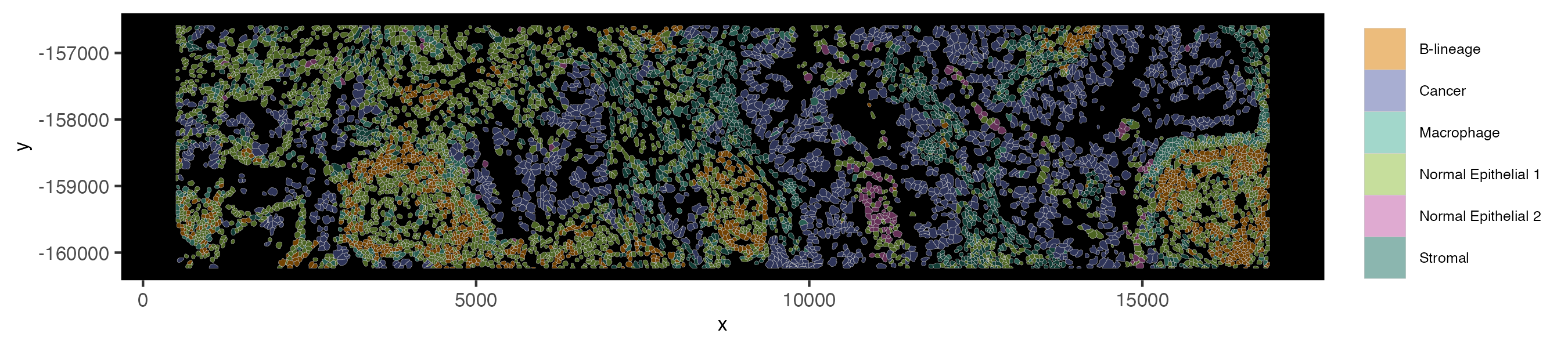
spatInSituPlotPoints(fov_join,
                     show_polygon = TRUE,
                     polygon_feat_type = 'cell',
                     polygon_color = 'grey',
                     polygon_line_size = 0.05,
                     polygon_fill = 'cell_types',
                     polygon_fill_as_factor = TRUE,
                     polygon_fill_code = viv10,
                     save_param = list(base_height = 2,
                                       save_name = '13_insitu_type'))
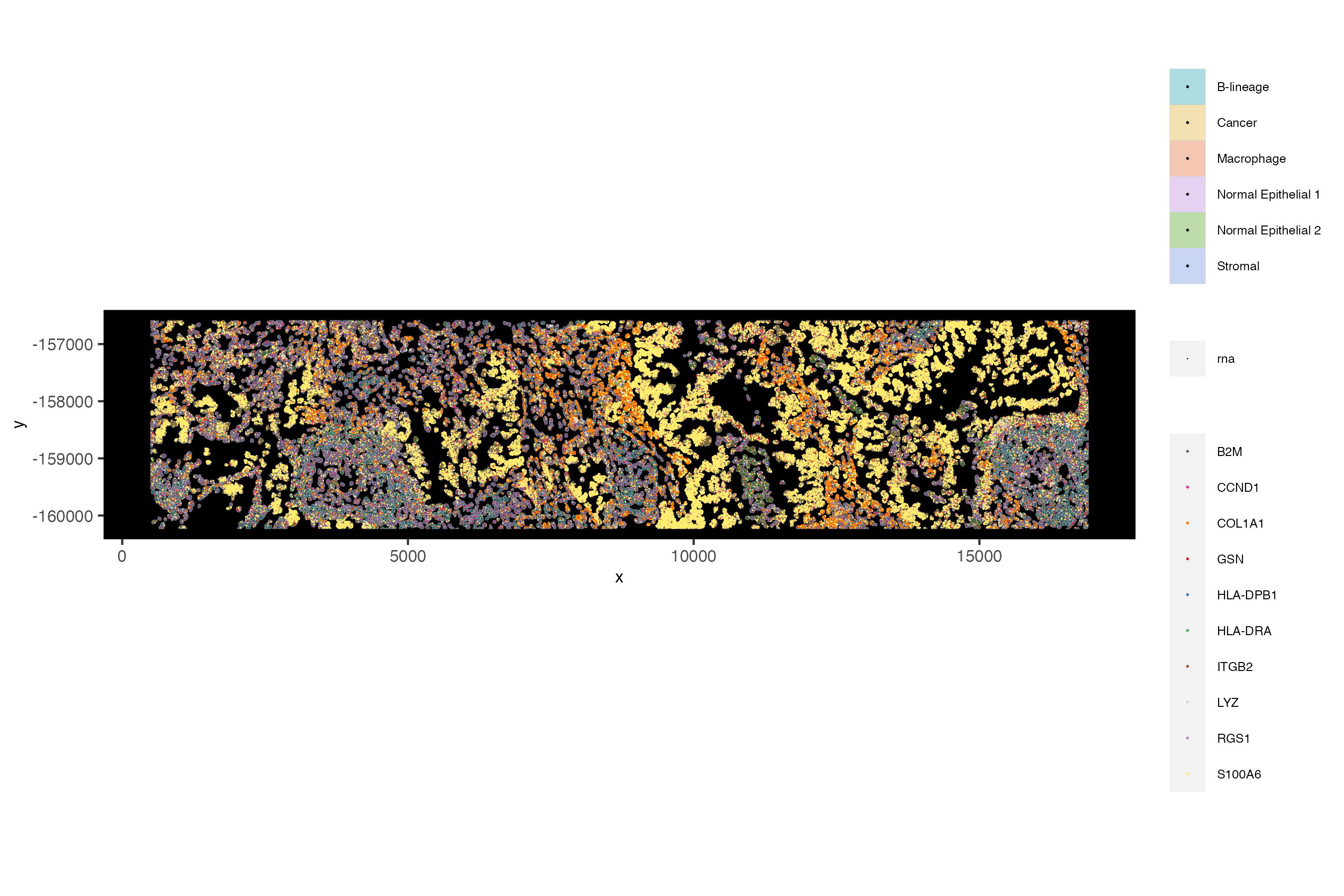
14. Interaction Changed Genes#
future::plan('multisession', workers = 4) # NOTE: Depending on your system this could take time

icf = findInteractionChangedFeats(gobject = fov_join,
                                  cluster_column = 'cell_types')

# Identify top ten interaction changed features
icf$ICFscores[type_int == 'hetero']$feats[1:10]

# Skip first two genes since they are too highly expressed
icf_plotfeats = icf$ICFscores[type_int == 'hetero']$feats[3:12]

# Visualize ICF expression
spatInSituPlotPoints(fov_join,
                     feats = list(icf_plotfeats),
                     point_size = 0.001,
                     show_polygon = TRUE,
                     polygon_feat_type = 'cell',
                     polygon_color = 'gray',
                     polygon_line_size = 0.05,
                     polygon_fill = 'cell_types',
                     polygon_fill_as_factor = TRUE,
                     polygon_fill_code = pal10,
                     save_param = list(base_height = 6,
                                       save_name = '14_ICF'))
15. Saving the giotto object#
Giotto uses many objects that include pointers to information that live
on disk instead of loading everything into memory. This includes both
giotto image objects (giottoImage, giottoLargeImage) and also
subcellular information (giottoPoints, giottoPolygon). When
saving the project as a .RDS or .Rdata, these pointers are
broken and can produce errors when loaded again.
saveGiotto() is a function that can save Giotto Suite projects into
a contained structured directory that can then be properly loaded again
later using loadGiotto().
saveGiotto(gobject = fov_join,
           foldername = 'new_folder_name',
           dir = '/directory/to/save/to/')
Session Info
sessionInfo()
# R version 4.2.1 (2022-06-23)
# Platform: x86_64-apple-darwin17.0 (64-bit)
# Running under: macOS Big Sur 11.6
#
# Matrix products: default
# LAPACK: /Library/Frameworks/R.framework/Versions/4.2/Resources/lib/libRlapack.dylib
#
# locale:
# [1] en_US.UTF-8/en_US.UTF-8/en_US.UTF-8/C/en_US.UTF-8/en_US.UTF-8
#
# attached base packages:
# [1] stats     graphics  grDevices utils     datasets  methods   base
#
# other attached packages:
# [1] Giotto_3.1   testthat_3.1.5 ggplot2_3.4.0
#
# loaded via a namespace (and not attached):
#   [1] utf8_1.2.2                  reticulate_1.26             R.utils_2.12.2
#   [4] tidyselect_1.2.0            htmlwidgets_1.5.4           grid_4.2.1
#   [7] BiocParallel_1.32.3         Rtsne_0.16                  devtools_2.4.5
#  [10] scatterpie_0.1.8            munsell_0.5.0               ScaledMatrix_1.6.0
#  [13] codetools_0.2-18            ragg_1.2.4                  statmod_1.4.37
#  [16] scran_1.24.1                future_1.29.0               miniUI_0.1.1.1
#  [19] withr_2.5.0                 colorspace_2.0-3            Biobase_2.56.0
#  [22] knitr_1.41                  rstudioapi_0.14             stats4_4.2.1
#  [25] SingleCellExperiment_1.18.1 listenv_0.8.0               MatrixGenerics_1.10.0
#  [28] labeling_0.4.2              GenomeInfoDbData_1.2.8      polyclip_1.10-4
#  [31] farver_2.1.1                rprojroot_2.0.3             parallelly_1.32.1
#  [34] vctrs_0.5.1                 generics_0.1.3              xfun_0.35
#  [37] R6_2.5.1                    doParallel_1.0.17           GenomeInfoDb_1.32.4
#  [40] clue_0.3-62                 rsvd_1.0.5                  locfit_1.5-9.6
#  [43] bitops_1.0-7                cachem_1.0.6                DelayedArray_0.24.0
#  [46] assertthat_0.2.1            promises_1.2.0.1            scales_1.2.1
#  [49] gtable_0.3.1                beachmat_2.14.0             globals_0.16.2
#  [52] processx_3.8.0              rlang_1.0.6                 systemfonts_1.0.4
#  [55] GlobalOptions_0.1.2         lazyeval_0.2.2              reshape2_1.4.4
#  [58] httpuv_1.6.6                tools_4.2.1                 usethis_2.1.6
#  [61] ellipsis_0.3.2              RColorBrewer_1.1-3          BiocGenerics_0.44.0
#  [64] rcartocolor_2.0.0           sessioninfo_1.2.2           Rcpp_1.0.9
#  [67] plyr_1.8.8                  sparseMatrixStats_1.10.0    zlibbioc_1.42.0
#  [70] purrr_0.3.5                 RCurl_1.98-1.9              ps_1.7.2
#  [73] prettyunits_1.1.1           dbscan_1.1-11               deldir_1.0-6
#  [76] GetoptLong_1.0.5            cowplot_1.1.1               urlchecker_1.0.1
#  [79] S4Vectors_0.36.0            SummarizedExperiment_1.26.1 ggrepel_0.9.2
#  [82] cluster_2.1.4               fs_1.5.2                    here_1.0.1
#  [85] magrittr_2.0.3              data.table_1.14.6           magick_2.7.3
#  [88] circlize_0.4.15             matrixStats_0.63.0          pkgload_1.3.1
#  [91] mime_0.12                   evaluate_0.18               xtable_1.8-4
#  [94] IRanges_2.32.0              shape_1.4.6                 compiler_4.2.1
#  [97] tibble_3.1.8                crayon_1.5.2                R.oo_1.25.0
# [100] htmltools_0.5.3             ggfun_0.0.8                 later_1.3.0
# [103] tidyr_1.2.1                 DBI_1.1.3                   tweenr_2.0.2
# [106] ComplexHeatmap_2.12.1       MASS_7.3-58.1               Matrix_1.5-3
# [109] brio_1.1.3                  cli_3.4.1                   R.methodsS3_1.8.2
# [112] parallel_4.2.1              metapod_1.4.0               igraph_1.3.5
# [115] GenomicRanges_1.48.0        pkgconfig_2.0.3             sp_1.5-1
# [118] terra_1.6-41                plotly_4.10.1               scuttle_1.6.3
# [121] foreach_1.5.2               dqrng_0.3.0                 XVector_0.36.0
# [124] stringr_1.4.1               callr_3.7.3                 digest_0.6.30
# [127] RcppAnnoy_0.0.20            rmarkdown_2.18              uwot_0.1.14
# [130] edgeR_3.38.4                DelayedMatrixStats_1.20.0   shiny_1.7.3
# [133] rjson_0.2.21                lifecycle_1.0.3             jsonlite_1.8.3
# [136] BiocNeighbors_1.14.0        desc_1.4.2                  viridisLite_0.4.1
# [139] limma_3.54.0                fansi_1.0.3                 pillar_1.8.1
# [142] lattice_0.20-45             fastmap_1.1.0               httr_1.4.4
# [145] pkgbuild_1.3.1              glue_1.6.2                  remotes_2.4.2
# [148] png_0.1-7                   iterators_1.0.14            bluster_1.6.0
# [151] ggforce_0.4.1               stringi_1.7.8               profvis_0.3.7
# [154] textshaping_0.3.6           BiocSingular_1.14.0         memoise_2.0.1
# [157] dplyr_1.0.10                irlba_2.3.5.1               future.apply_1.10.0