Data Processing#

Date:: 4/12/23

1 Dataset explanation#

After creating the Giotto object, it must be prepared for downstream analysis. This tutorial walks through filtering, normalizing, adjusting for batch effects, adding statistics and metadata to a Giotto object, as well as high efficiency options for data processing.

This tutorial uses a SeqFISH+ dataset of a murine cortex and subventrical zone. A complete walkthrough of that dataset can be found here. To download the data used to create the Giotto Object below, please ensure that wget is installed locally.

This dataset contains multiple field of views; here, a workflow to bring the FOVs together for holistic analysis is illustrated, and then a subset of the Giotto Object is taken to analyze the cortex.

2 Start Giotto#

# Ensure Giotto Suite is installed
if(!"Giotto" %in% installed.packages()) {
  devtools::install_github("drieslab/Giotto@suite")
}
library(Giotto)

# Ensure Giotto Data is installed
if(!"GiottoData" %in% installed.packages()) {
  devtools::install_github("drieslab/GiottoData")
}
library(GiottoData)

# Ensure the Python environment for Giotto has been installed
genv_exists = checkGiottoEnvironment()
if(!genv_exists){
  # The following command need only be run once to install the Giotto environment
  installGiottoEnvironment()
}

3 Create a Giotto object#

# Specify path from which data may be retrieved/stored
data_directory = paste0(getwd(),'/gobject_processing_data/')
# alternatively, "/path/to/where/the/data/lives/"

# Specify path to which results may be saved
results_directory = paste0(getwd(),'/gobject_processing_results/')
# alternatively, "/path/to/store/the/results/"

# Optional: Specify a path to a Python executable within a conda or miniconda
# environment. If set to NULL (default), the Python executable within the previously
# installed Giotto environment will be used.
my_python_path = NULL # alternatively, "/local/python/path/python" if desired.

getSpatialDataset(dataset = 'seqfish_SS_cortex', directory = data_directory, method = 'wget')

# Set Giotto instructions
instrs = createGiottoInstructions(save_plot = TRUE,
                                  show_plot = FALSE,
                                  save_dir = results_directory,
                                  python_path = my_python_path)

# Create Giotto object by providing paths
expr_path = paste0(data_directory, "cortex_svz_expression.txt")
loc_path = paste0(data_directory, "cortex_svz_centroids_coord.txt")
meta_path = paste0(data_directory, "cortex_svz_centroids_annot.txt")


# This dataset contains multiple field of views which need to be stitched together.

# First, merge location and additional metadata
SS_locations = data.table::fread(loc_path)
cortex_fields = data.table::fread(meta_path)
SS_loc_annot = data.table::merge.data.table(SS_locations, cortex_fields, by = 'ID')
SS_loc_annot[, ID := factor(ID, levels = paste0('cell_',1:913))]
data.table::setorder(SS_loc_annot, ID)

# Create a file with offset information
my_offset_file = data.table::data.table(field = c(0, 1, 2, 3, 4, 5, 6),
                                        x_offset = c(0, 1654.97, 1750.75, 1674.35, 675.5, 2048, 675),
                                        y_offset = c(0, 0, 0, 0, -1438.02, -1438.02, 0))

# Create a file to stitch the multiple fields of view together
stitch_file = stitchFieldCoordinates(location_file = SS_loc_annot,
                                     offset_file = my_offset_file,
                                     cumulate_offset_x = T,
                                     cumulate_offset_y = F,
                                     field_col = 'FOV',
                                     reverse_final_x = F,
                                     reverse_final_y = T)

stitch_file    = stitch_file[,.(ID, X_final, Y_final)]
stitch_file$ID = as.character(stitch_file$ID) # ID must be a character vector
my_offset_file = my_offset_file[,.(field, x_offset_final, y_offset_final)]

# Create Giotto object
testobj <- createGiottoObject(expression = expr_path,
                              spatial_locs = stitch_file,
                              offset_file = my_offset_file,
                              instructions = instrs)

# Add additional annotation if wanted
testobj = addCellMetadata(testobj,
                          new_metadata = cortex_fields,
                          by_column = T,
                          column_cell_ID = 'ID')

# Subset data to the cortex field of views in a new Giotto object
cell_metadata = getCellMetadata(testobj)[]
cortex_cell_ids = cell_metadata[FOV %in% 0:4]$cell_ID
testobj = subsetGiotto(testobj, cell_ids = cortex_cell_ids)

Since subsetGiotto returns a Giotto object, multiple different objects may be created to store subsets. For the purposes of this tutorial, only the cortex FOVs will be considered, which is why the original Giotto Object has been overwritten upon calling subsetGiotto.

4 Filter the Giotto Object#

The Giotto object may be filtered based on:

expression_thresholds sets a minimum threshold expression level
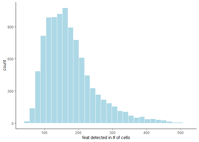
feat_det_in_min_cells sets a threshold of the number of cells that must include a feature in order to keep that feature in the dataset
min_det_feats_per_cell sets a threshold of the number of features expressed by a cell in order to keep that cell in the dataset

The distribution of feature expression can inform stringency of filter parameters, and can be displayed for both cells and features by calling filterDistributions and specifying the ‘detection’ parameter accordingly:

filterDistributions(testobj, detection = 'cells')

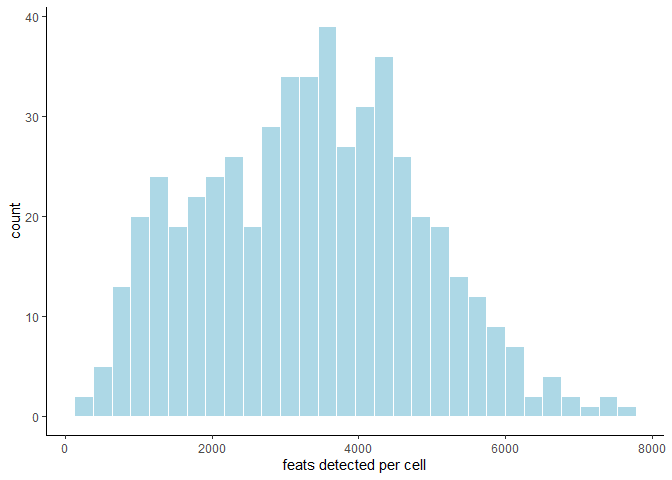
filterDistributions(testobj, detection = 'feats')

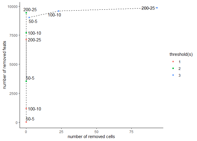
filterCombinations may be used to test how different filtering parameters will affect the number of cells and features in the filtered data:

filterCombinations(testobj,
                   expression_thresholds = c(1,2, 3),
                   feat_det_in_min_cells = c(50, 100, 200),
                   min_det_feats_per_cell = c(5, 10, 25))

When a consensus on appropriate filtering parameters has been reached, provide the arguments to filterGiotto.

testobj <- filterGiotto(gobject = testobj,
                        expression_threshold = 1,
                        feat_det_in_min_cells = 100,
                        min_det_feats_per_cell = 10)

5 Normalize Raw Counts Data#

There are three methods of normalization supported by Giotto.

The ‘standard’ method (default) normalizes the data by total library size and a custom scale factor, then log transforms and z-scores the data by cells or genes, specified by scale_order.

# normalize to scale expression values of the Giotto object using the standard method, z-scoring feats over cells
testobj <- normalizeGiotto(gobject = testobj,
                           norm_methods = 'standard',
                           scale_feats = TRUE,
                           scalefactor = 6000,
                           scale_order = 'first_feats', # Default, alternatively 'first_cells'
                           verbose = T)

The ‘pearson_resid’ method uses the Lause/Kobak et al. method. First, expected values are calculated based on Pearson correlations. Next, z-scores are calculated based on observed and expected values. Note that normalizing with this method will save the data within the “scaled” expression slot, NOT the “normalized” slot.

# normalize to scale expression values of the Giotto object using the pearson residual method
testobj <- normalizeGiotto(gobject = testobj,
                           norm_methods = 'pearson_resid',
                           scale_feats = TRUE,
                           scalefactor = 6000,
                           verbose = T)

The ‘osmFISH’ method is intended for in-situ RNA data and uses the normalization method described by Codeluppi et al. Feature (gene) counts are individually normalized by the total feature count, and then are multiplied by the total number of features. Then, cells are individually normalized by dividing the normalized feature counts by the total feature counts per cell, and then are scaled by the total number of cells.

Since the data in this tutorial is not in-situ RNA data, this method will not be shown here. It may be utilized by specifying the norm_methods argument as ‘osmFISH’.

6 Add Statistics and Metadata to the Giotto Object#

The function addStatistics will add the following statistics to cell metadata:

nr_feats: Denotes how many features are detected per cell
perc_feats: Denotes the percentage of features detected per cell
total_expr: Shows the total sum of feature expression per cell

It will also add the following statistics to feature metadata:

nr_cells: Denotes how many cells in which the feature is detected
per_cells: Denotes the percentage of cells in which the feature is detected
total_expr: Shows the total sum of feature expression in all cells
mean_expr: Average feature expression in all cells
mean_expr_det: Average feature expression in cells with detectable levels of the feature

# Add gene & cell statistics to the Giotto object using the data normalized with the standard method
testobj <- addStatistics(gobject = testobj, expression_values = 'normalized')

# Accessors:

cell_metadata_cortex <- getCellMetadata(testobj)
## Convert from cellMetaObj to data.table
cell_metadata_cortex <- cell_metadata_cortex[]

## Retrieve a data.table in one step instead of a featMetaObj
feature_metadata_cortex <- getFeatureMetadata(testobj, output = "data.table")

addFeatsPerc can be used to detect the percentage of features in each cell within a given gene family (ie. mitochondrial genes, ribosomal genes)

#Calculate the percentage of BMP genes per cell
bmp_genes = grep('Bmp', x = feature_metadata_cortex$feat_ID, value = TRUE)
testobj <- addFeatsPerc(testobj,
                        expression_values = 'normalized',
                        feats = bmp_genes,
                        vector_name = "perc_bmp")

7 Adjust Expression Matrix#

Adjust expression matrix for known batch effects or technological covariates.

# Since there are no known batch effects, the number of features detected per cell
# will be regressed out so that covariates will not effect further analyses.

testobj <- adjustGiottoMatrix(gobject = testobj,
                            expression_values = c('normalized'),
                            covariate_columns = 'nr_feats')

8 High Efficiency Data Processing#

processGiotto completes the filtering, normalization, statistical, and adjustment steps of data processing in one single step; this is ideal for faster processing.

Since adjustment is not necessary for every dataset, adjust_params may be set to NULL to skip this processing step. All other arguments are user-determined; default arguments will apply to all steps if no arguments are provided.

testobj <- processGiotto(testobj,
                         filter_params = list(expression_threshold = 1,
                                              feat_det_in_min_cells = 100,
                                              min_det_feats_per_cell = 10),
                         norm_params = list(norm_methods = 'standard',
                                            scale_feats = TRUE,
                                            scalefactor = 6000),
                         stat_params = list(expression_values = 'normalized'),
                         adjust_params = list(expression_values = c('normalized'),
                                              covariate_columns = 'nr_feats'))

9 Session Info#

sessionInfo()

R version 4.2.2 (2022-10-31 ucrt)
Platform: x86_64-w64-mingw32/x64 (64-bit)
Running under: Windows 10 x64 (build 22621)

Matrix products: default

locale:
[1] LC_COLLATE=English_United States.utf8
[2] LC_CTYPE=English_United States.utf8
[3] LC_MONETARY=English_United States.utf8
[4] LC_NUMERIC=C
[5] LC_TIME=English_United States.utf8

attached base packages:
[1] stats     graphics  grDevices utils     datasets  methods   base

other attached packages:
[1] GiottoData_0.1.0 Giotto_3.2.1

loaded via a namespace (and not attached):
 [1] reticulate_1.26   tidyselect_1.2.0  terra_1.7-18      xfun_0.38
 [5] lattice_0.20-45   colorspace_2.1-0  vctrs_0.6.1       generics_0.1.3
 [9] htmltools_0.5.4   yaml_2.3.7        utf8_1.2.3        rlang_1.1.0
[13] pillar_1.9.0      glue_1.6.2        withr_2.5.0       rappdirs_0.3.3
[17] lifecycle_1.0.3   munsell_0.5.0     gtable_0.3.3      ragg_1.2.4
[21] codetools_0.2-18  evaluate_0.20     labeling_0.4.2    knitr_1.42
[25] fastmap_1.1.0     parallel_4.2.2    fansi_1.0.4       Rcpp_1.0.10
[29] scales_1.2.1      limma_3.54.2      jsonlite_1.8.3    farver_2.1.1
[33] systemfonts_1.0.4 textshaping_0.3.6 ggplot2_3.4.1     png_0.1-7
[37] digest_0.6.30     dplyr_1.1.1       ggrepel_0.9.2     grid_4.2.2
[41] rprojroot_2.0.3   cowplot_1.1.1     here_1.0.1        cli_3.4.1
[45] tools_4.2.2       magrittr_2.0.3    tibble_3.2.1      pkgconfig_2.0.3
[49] Matrix_1.5-1      data.table_1.14.6 rmarkdown_2.21    rstudioapi_0.14
[53] R6_2.5.1          compiler_4.2.2