Resolve Bioscience Breast Cancer Subcellular#
# Ensure Giotto Suite is installed.
if(!"Giotto" %in% installed.packages()) {
  devtools::install_github("drieslab/Giotto@suite")
}

# Ensure GiottoData, a small, helper module for tutorials, is installed.
if(!"GiottoData" %in% installed.packages()) {
  devtools::install_github("drieslab/GiottoData")
}
library(Giotto)
# Ensure the Python environment for Giotto has been installed.
genv_exists = checkGiottoEnvironment()
if(!genv_exists){
  # The following command need only be run once to install the Giotto environment.
  installGiottoEnvironment()
}
Start Giotto#
library(Giotto)
library(GiottoData)

# 1. set working directory
my_working_dir = '/path/to/directory'

# Optional: Specify a path to a Python executable within a conda or miniconda
# environment. If set to NULL (default), the Python executable within the previously
# installed Giotto environment will be used.
my_python_path = NULL # alternatively, "/local/python/path/python" if desired.
Input Files#
## provide path to resolve bioscience folder
data_path = '/path/to/Resolve_bioscience_cancer'


# 1. original image as png
original_DAPI_image = paste0(data_path, '/', 'sample2_DAPI.jpg')

# 2. input cell segmentation as mask file
# can also be provided as a 3-column polygon file
# to be used as image background AND to store segmentations as polygons
# can be obtained through Fiji / QuPath / Ilastik / Cellpose / ...
segmentation_mask = paste0(data_path, '/', 'Mask3.png')

# 3. input features coordinates
tx_coord = fread(paste0(data_path, '/', 'data_sample2.txt'))
colnames(tx_coord) = c('x', 'y', 'z', 'gene_id')
tx_coord = tx_coord[,.(x, y, gene_id)]
Part 1: Create Subcellular Giotto Object#
testobj = createGiottoObjectSubcellular(gpoints = list('rna' = tx_coord),
                    gpolygons = list('cell' = segmentation_mask),
                    instructions = instrs,
                    verbose = FALSE,
                    cores = 32)
Part 2: Create Spatial Locations#
# centroids are now used to provide the spatial locations (centroid of each cell)
# needed for certain downstream spatial analyses
testobj = addSpatialCentroidLocations(testobj,
                    poly_info = 'cell')
Part 3: Add Image Information#
# create Giotto images
DAPI_image = createGiottoImage(gobject = testobj,
                name = 'DAPI',
                do_manual_adj = T,
                xmax_adj = 0,ymax_adj = 0,
                xmin_adj = 0,ymin_adj = 0,
                image_transformations = 'flip_x_axis',
                mg_object = original_DAPI_image)

segm_image = createGiottoImage(gobject = testobj,
                name = 'segmentation',
                do_manual_adj = T,
                xmax_adj = 0,ymax_adj = 0,
                xmin_adj = 0,ymin_adj = 0,
                image_transformations = 'flip_x_axis',
                mg_object = segmentation_mask)

# add images to Giotto object
testobj = addGiottoImage(testobj,
            images = list(DAPI_image, segm_image))

# provides an overview of available images
showGiottoImageNames(testobj)
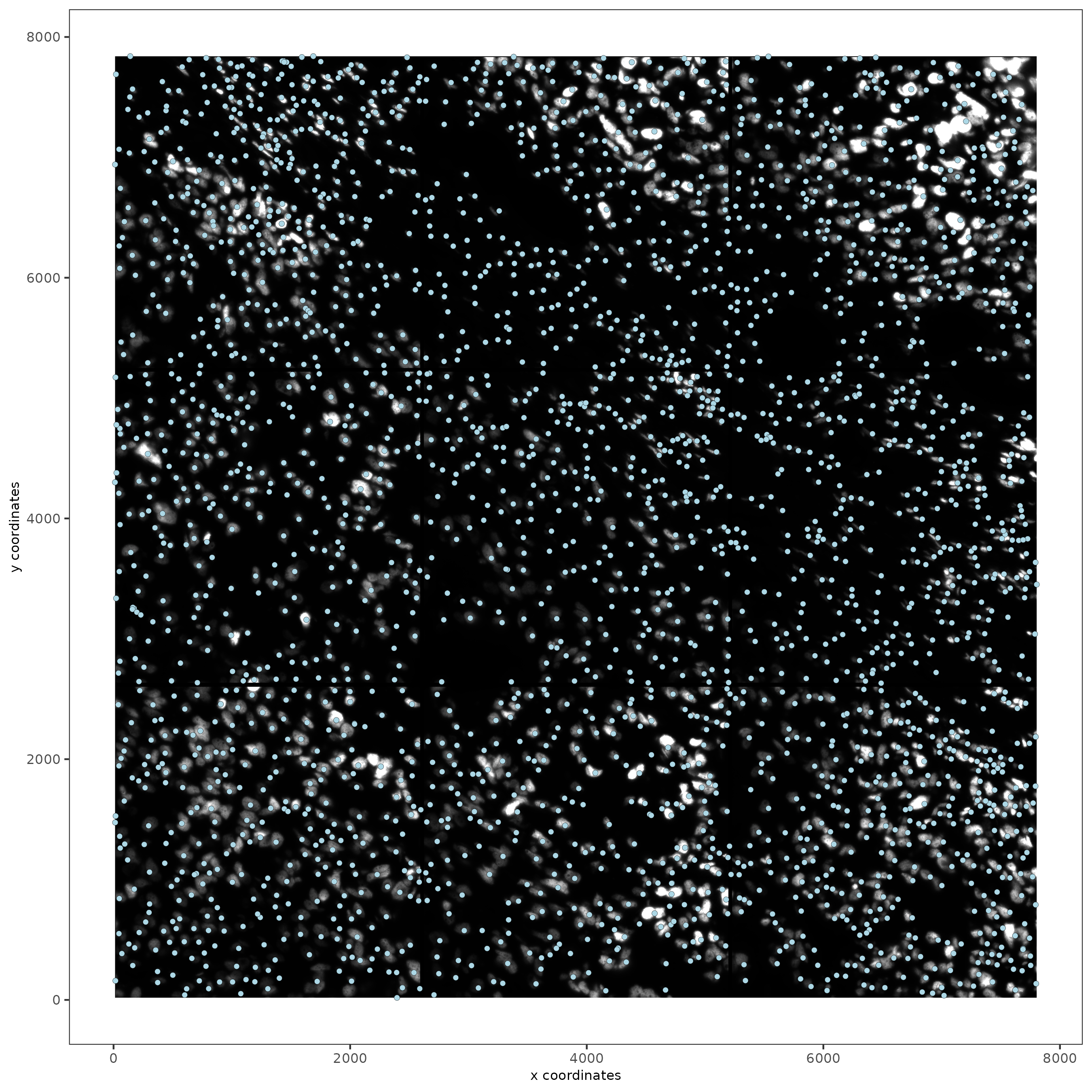
Part 4: Visualize Original Images#
# visualize overlay of calculated cell centroid with original image and segmentation mask file
 # by setting show_plot to FALSE and save_plot to TRUE you can save quite some time when creating plots
 # with big images it sometimes takes quite long for R/Rstudio to render them
 spatPlot2D(gobject = testobj, image_name = 'DAPI', point_size = 1.5)
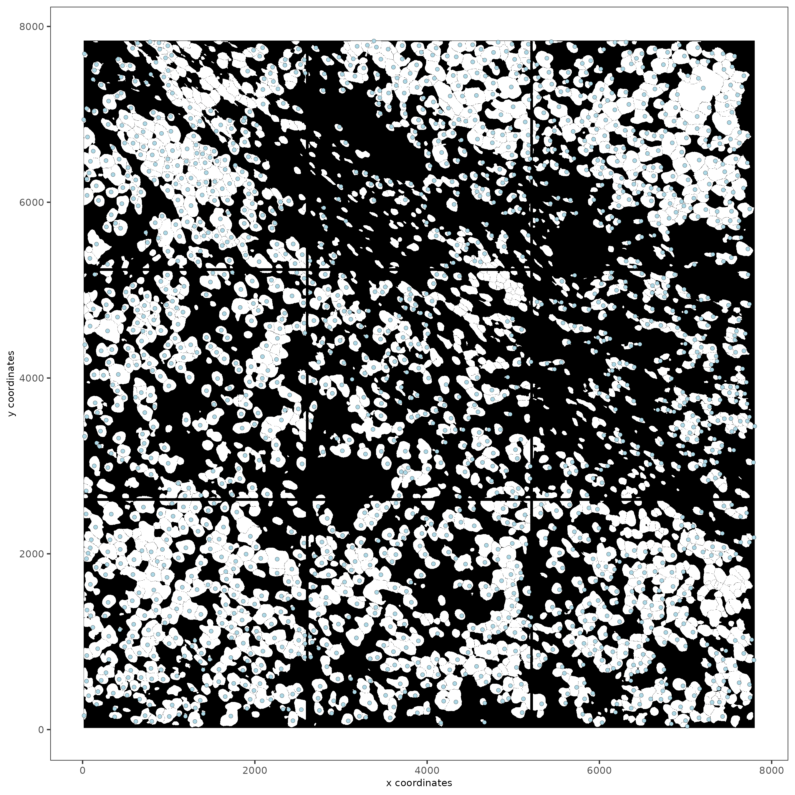
spatPlot2D(gobject = testobj, image_name = 'segmentation', point_size = 1.5)
Part 5: Calculate Cell Shape Overlap#
tictoc::tic()
testobj = calculateOverlap(testobj,
            method = 'parallel',
            x_step = 1000,
            y_step = 1000,
            poly_info = 'cell',
            feat_info = 'rna')
tictoc::toc()
#convert overlap to matrix
testobj = overlapToMatrix(testobj,
            poly_info = 'cell',
            feat_info = 'rna',
            name = 'raw')
Part 6: Filter Data#
# features can be filtered individually
# cells will be filtered across features
# first filter on rna
subc_test <- filterGiotto(gobject = testobj,
expression_threshold = 1,
feat_det_in_min_cells = 20,
min_det_feats_per_cell = 5)
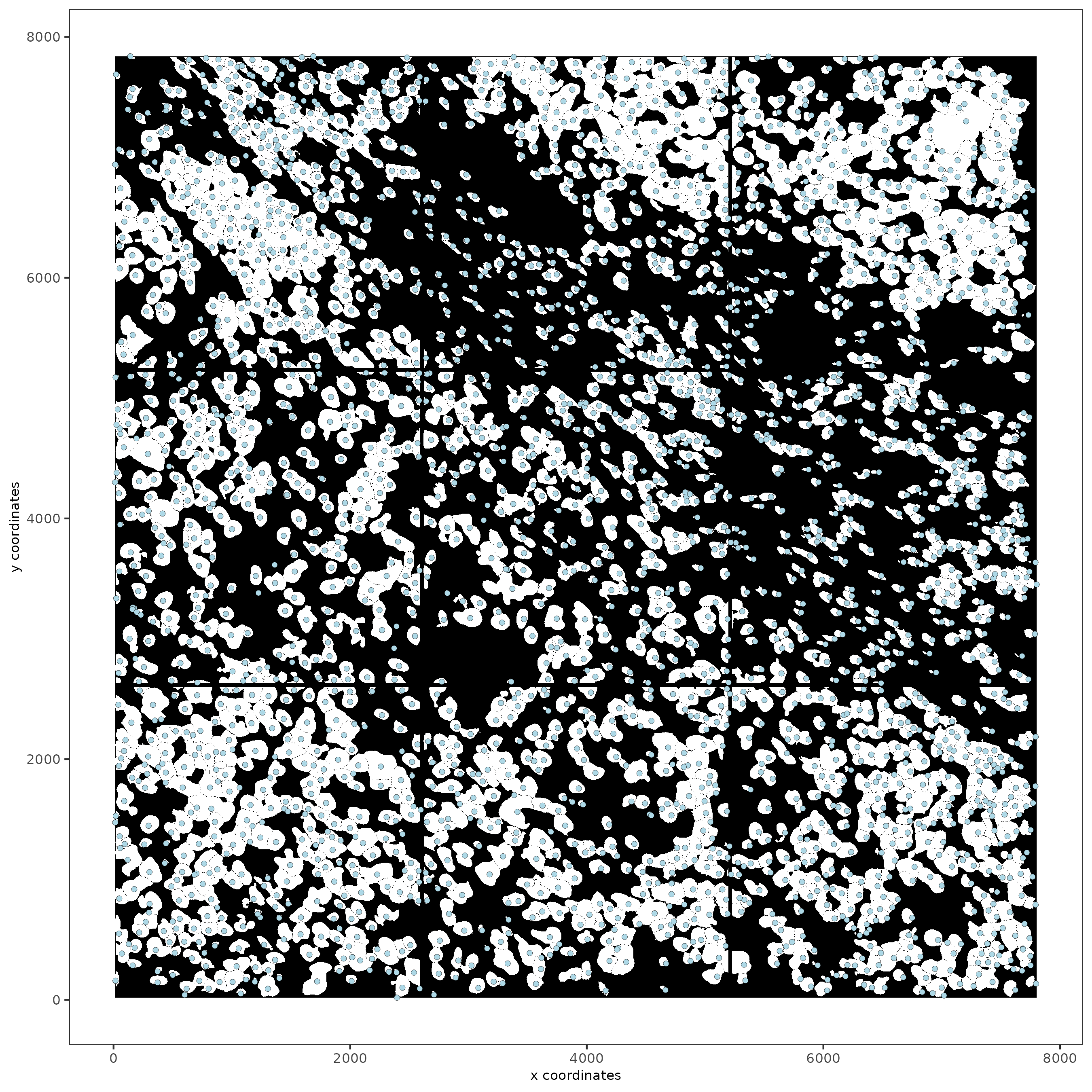
spatPlot2D(gobject = subc_test,
image_name = 'segmentation', show_image = TRUE,
point_size = 1.5)
# rna data, default.
 # other feature modalities can be processed and filtered in an anologous manner
 subc_test <- normalizeGiotto(gobject = subc_test, scalefactor = 6000, verbose = T)
 subc_test <- addStatistics(gobject = subc_test)
 subc_test <- adjustGiottoMatrix(gobject = subc_test,
                 expression_values = c('normalized'),
                 covariate_columns = c('nr_feats', 'total_expr'))

 subc_test <- normalizeGiotto(gobject = subc_test, norm_methods = 'pearson_resid', update_slot = 'pearson')
 showGiottoExpression(subc_test)
Part 8: Dimension Reduction#
# Find highly valuable Features

# typical way of calculating HVF
subc_test <- calculateHVF(gobject = subc_test, HVFname= 'hvg_orig')
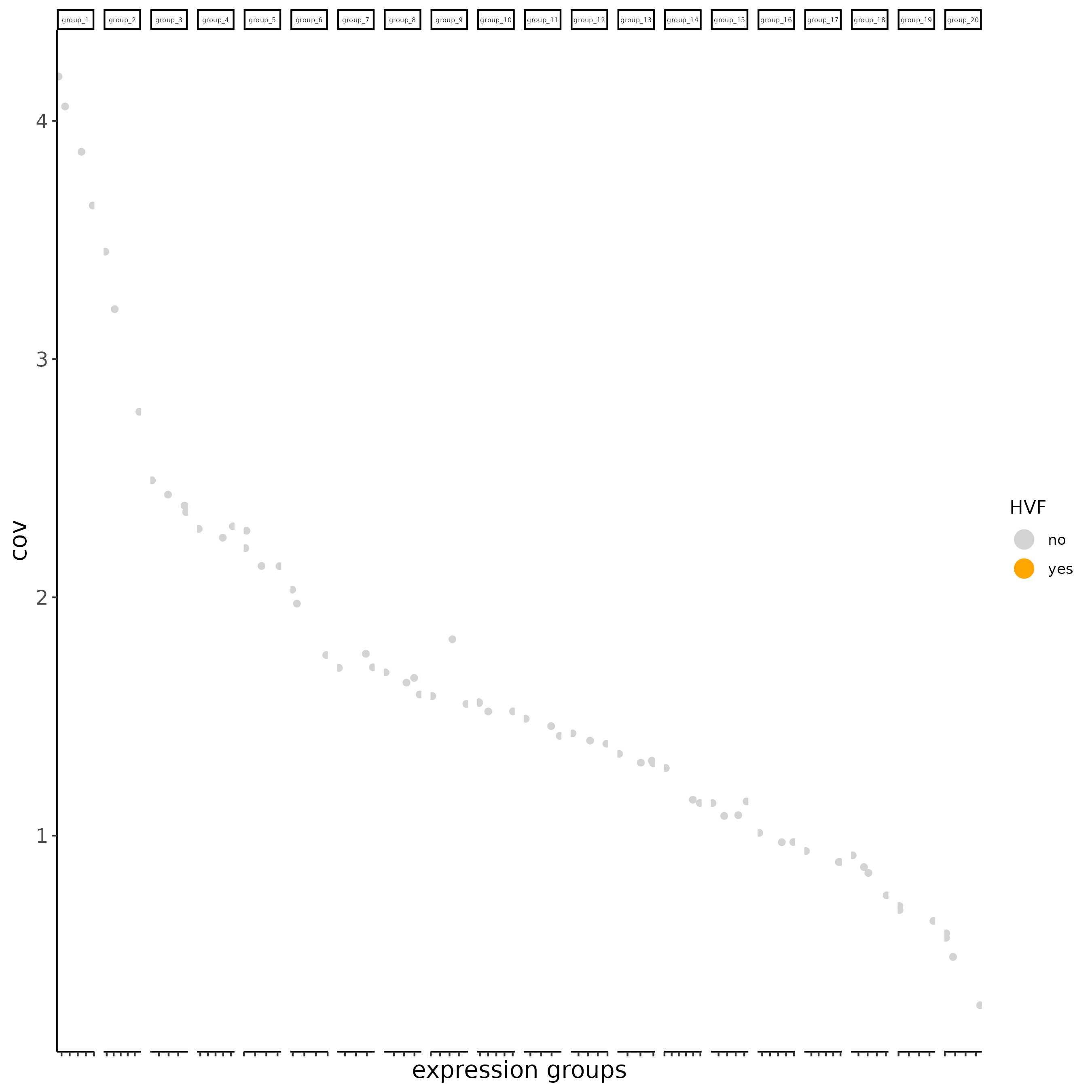
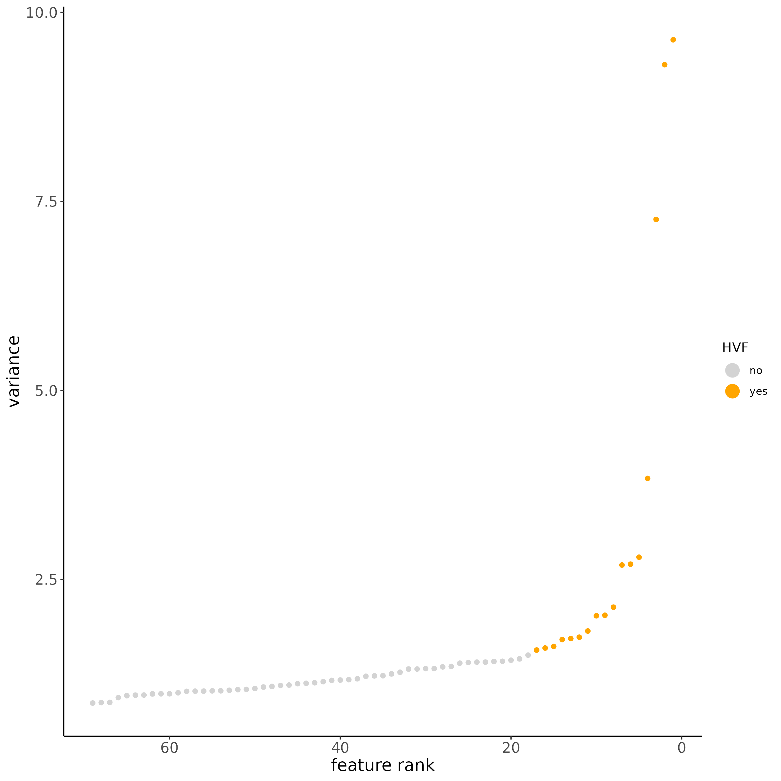
# new method based on variance of pearson residuals for each gene
subc_test <- calculateHVF(gobject = subc_test,
            method = 'var_p_resid', expression_values = 'pearson',
            show_plot = T)
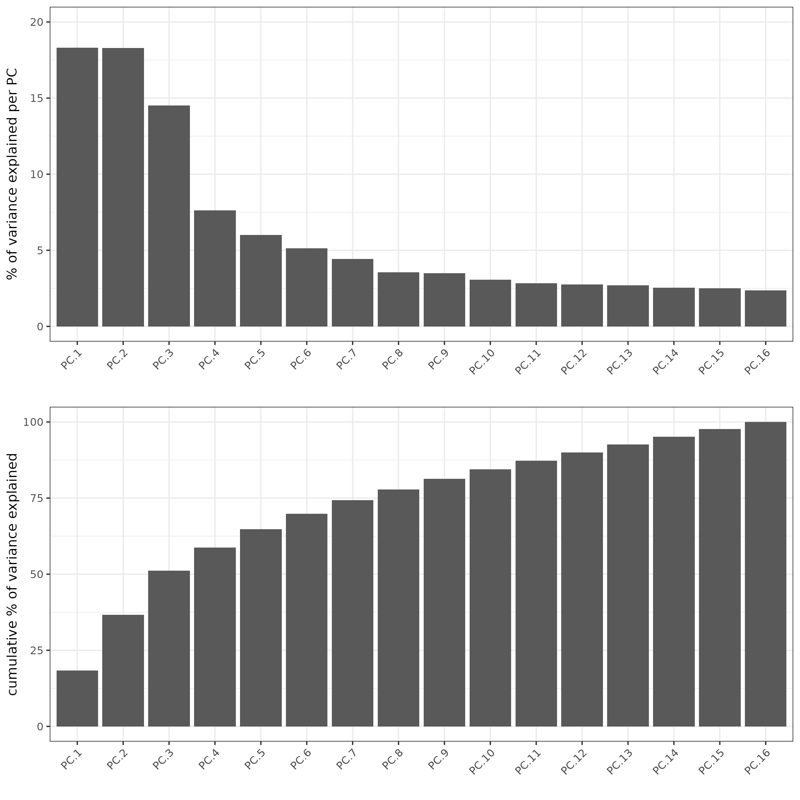
#run PCA
subc_test <- runPCA(gobject = subc_test,
            expression_values = 'pearson',
            scale_unit = F, center = F)

screePlot(subc_test, ncp = 20)
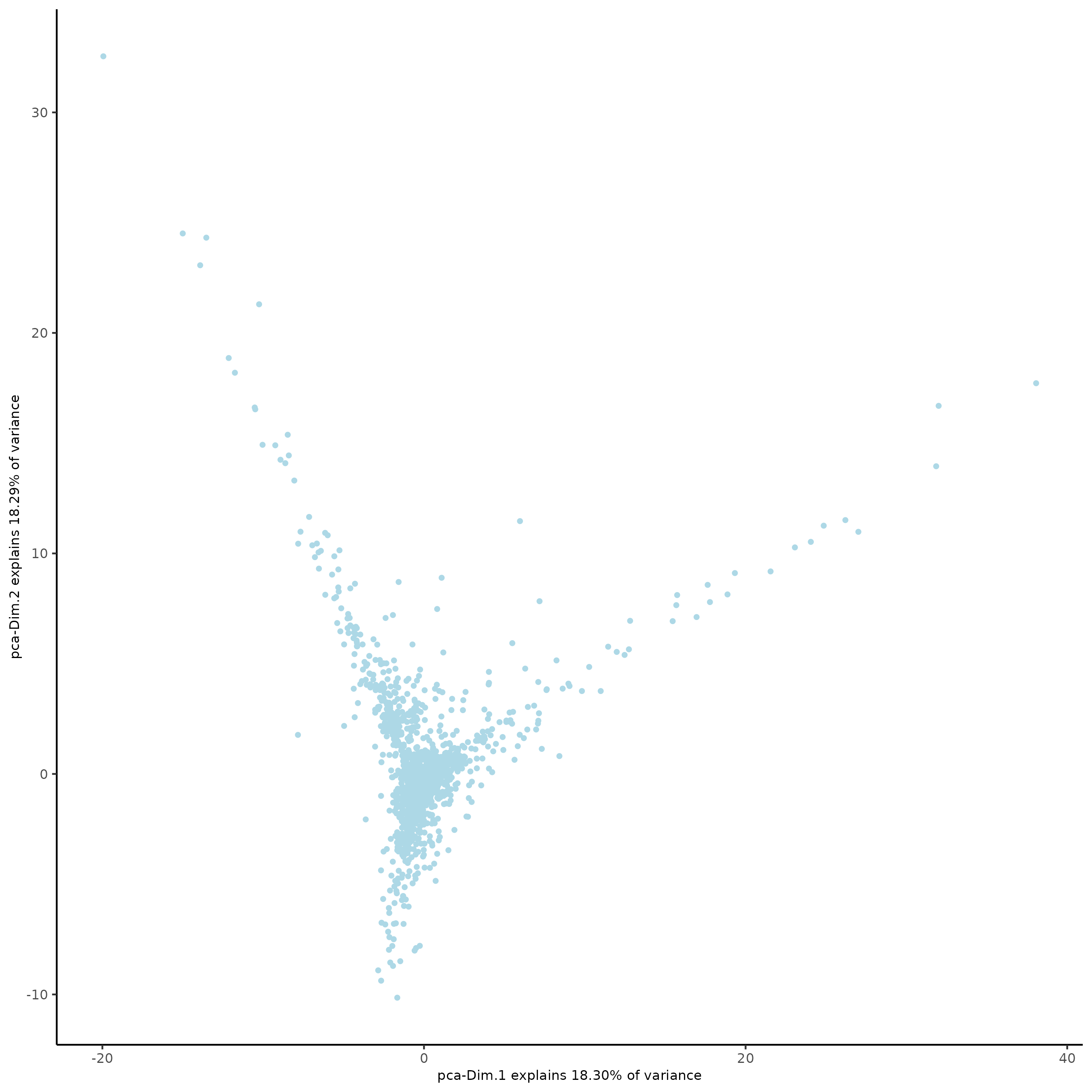
plotPCA(subc_test,
    dim1_to_use = 1,
    dim2_to_use = 2)
# run UMAP
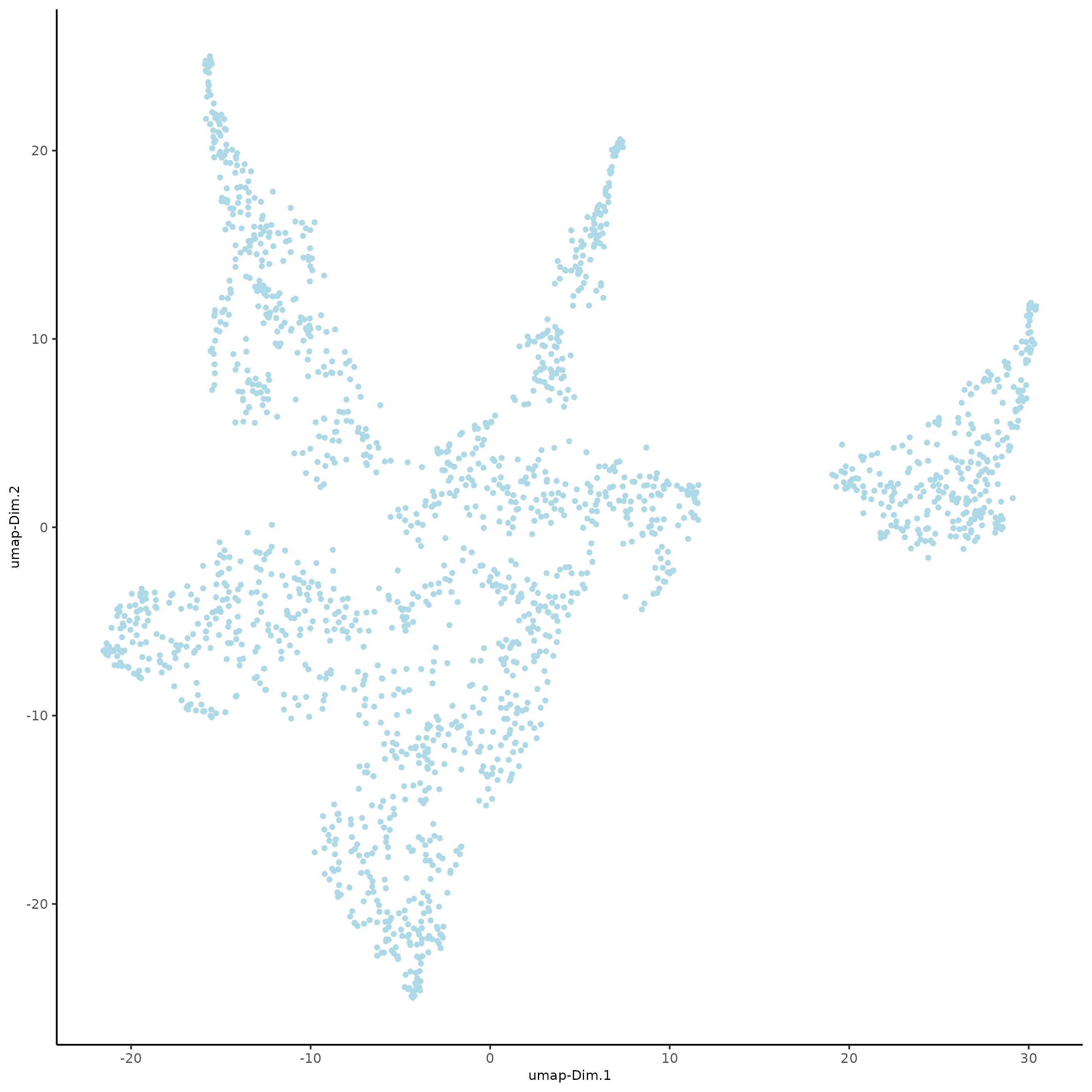
subc_test <- runUMAP(subc_test, dimensions_to_use = 1:5, n_threads = 2)
plotUMAP(gobject = subc_test)
Part 9: Cluster#
subc_test <- createNearestNetwork(gobject = subc_test, dimensions_to_use = 1:5, k = 5)
subc_test <- doLeidenCluster(gobject = subc_test, resolution = 0.05, n_iterations = 1000, name = 'leiden_0.05')
# Create color palettes, or proceed with Giotto defaults
devtools::install_github("alyssafrazee/RSkittleBrewer")
colorcode = lacroix_palette(type = "paired")
featcolor = lacroix_palette("KeyLime", type = "discrete")
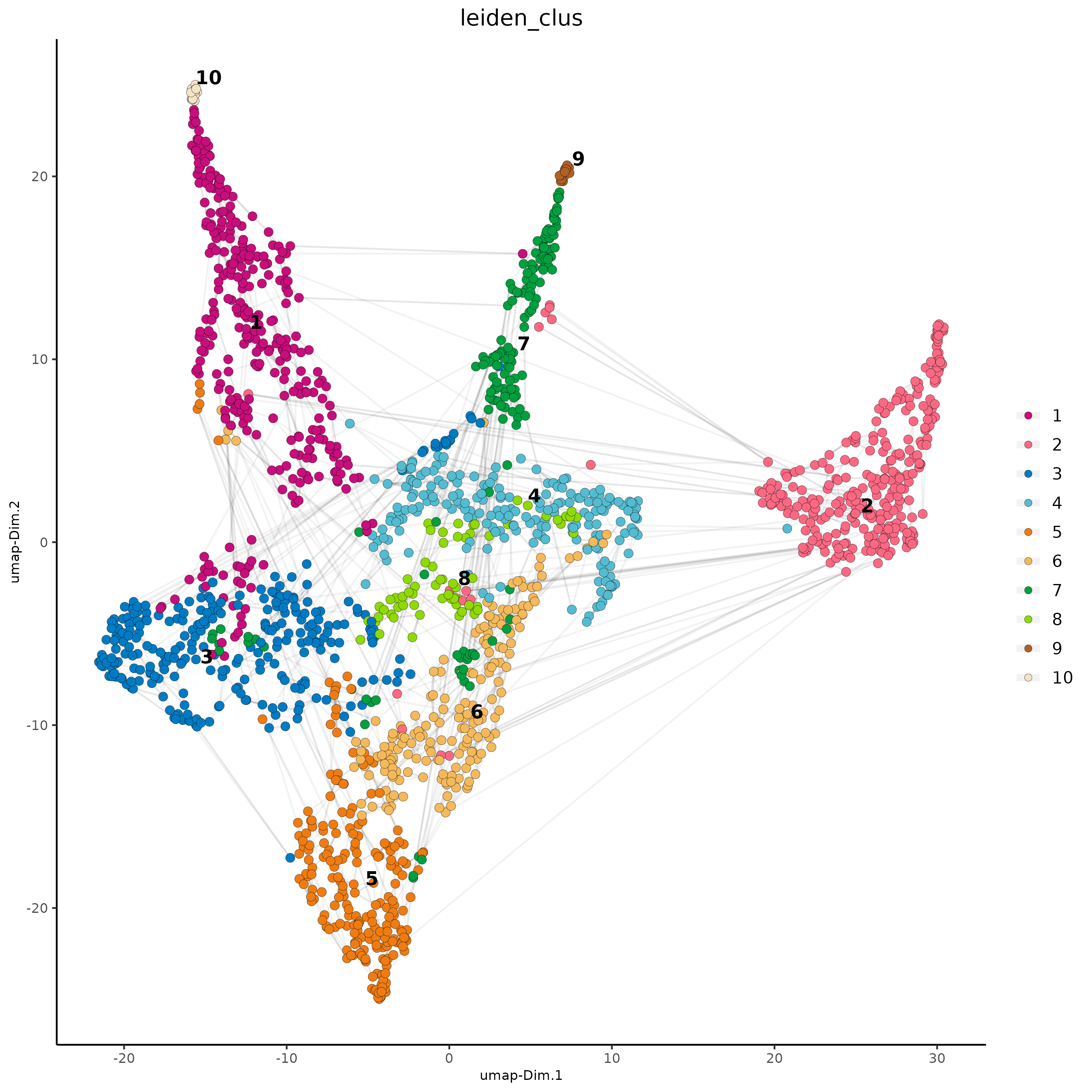
# visualize UMAP cluster results
plotUMAP(gobject = subc_test, cell_color = 'leiden_clus',
show_NN_network = T, point_size = 2.5, cell_color_code = colorcode)
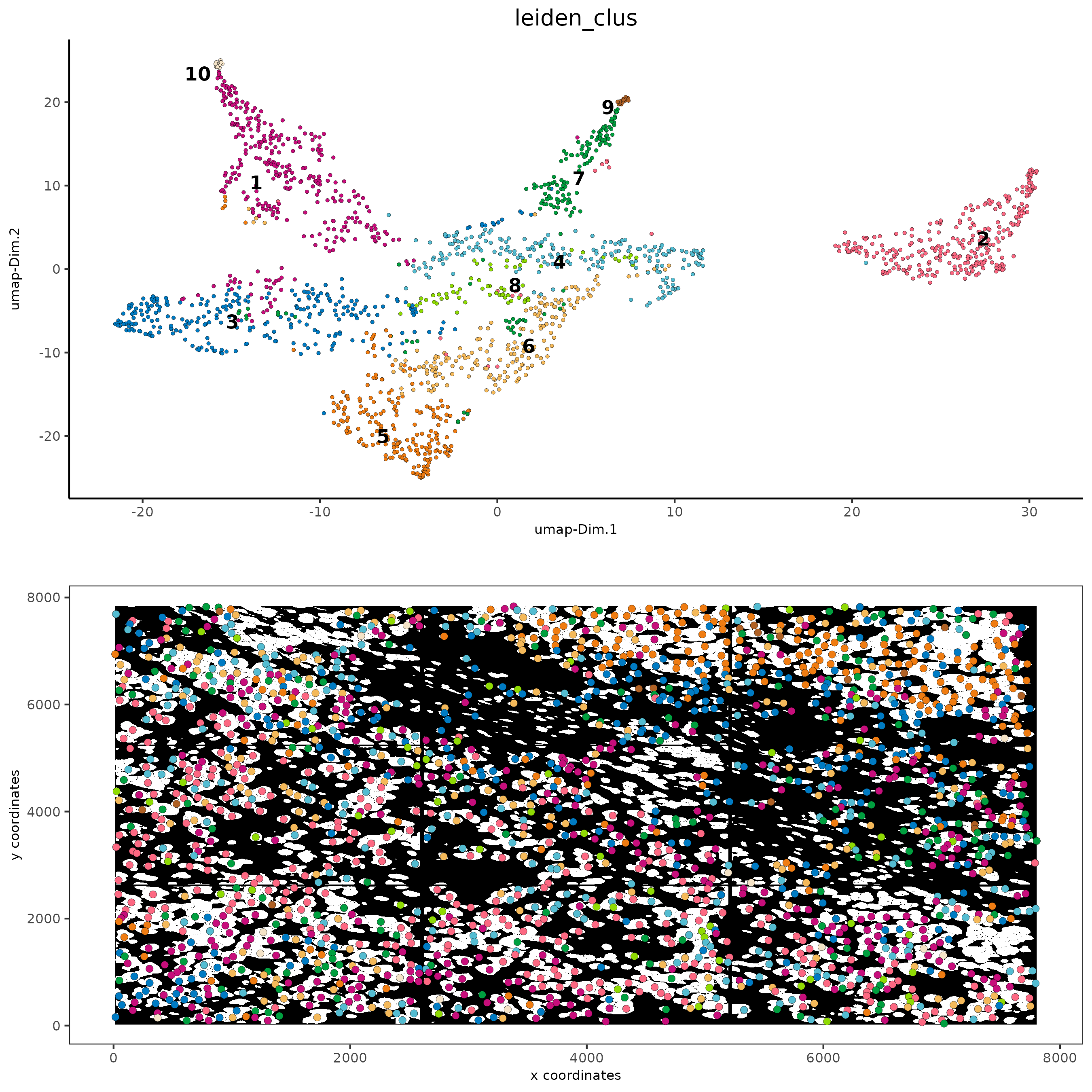
# visualize UMAP and spatial results
spatDimPlot2D(gobject = subc_test,
        show_image = T, image_name = 'segmentation',
        cell_color = 'leiden_clus',
        spat_point_size = 2, cell_color_code = colorcode)
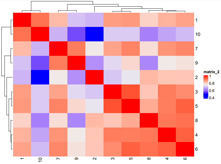
# Plot a cluster heatmap
showClusterHeatmap(gobject = subc_test, cluster_column = 'leiden_clus',
        save_param = list(save_format = 'pdf',base_height = 6, base_width = 8, units = 'cm'))
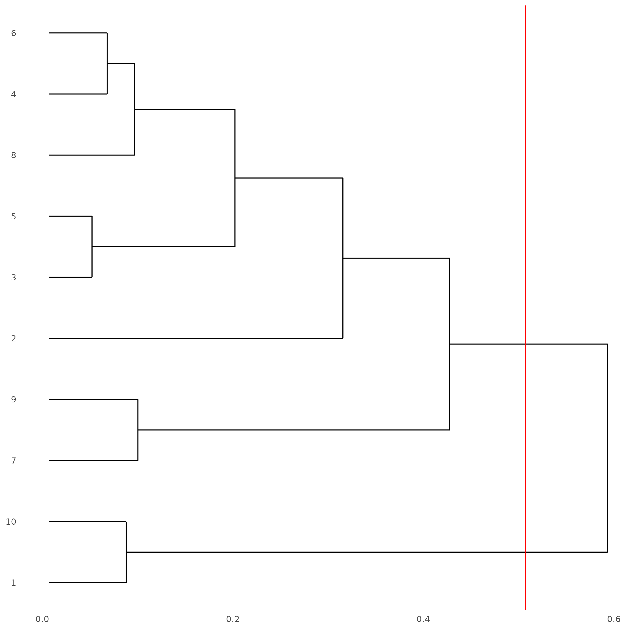
# See cluster relationships in a dendogram
showClusterDendrogram(subc_test, h = 0.5, rotate = T, cluster_column = 'leiden_clus')
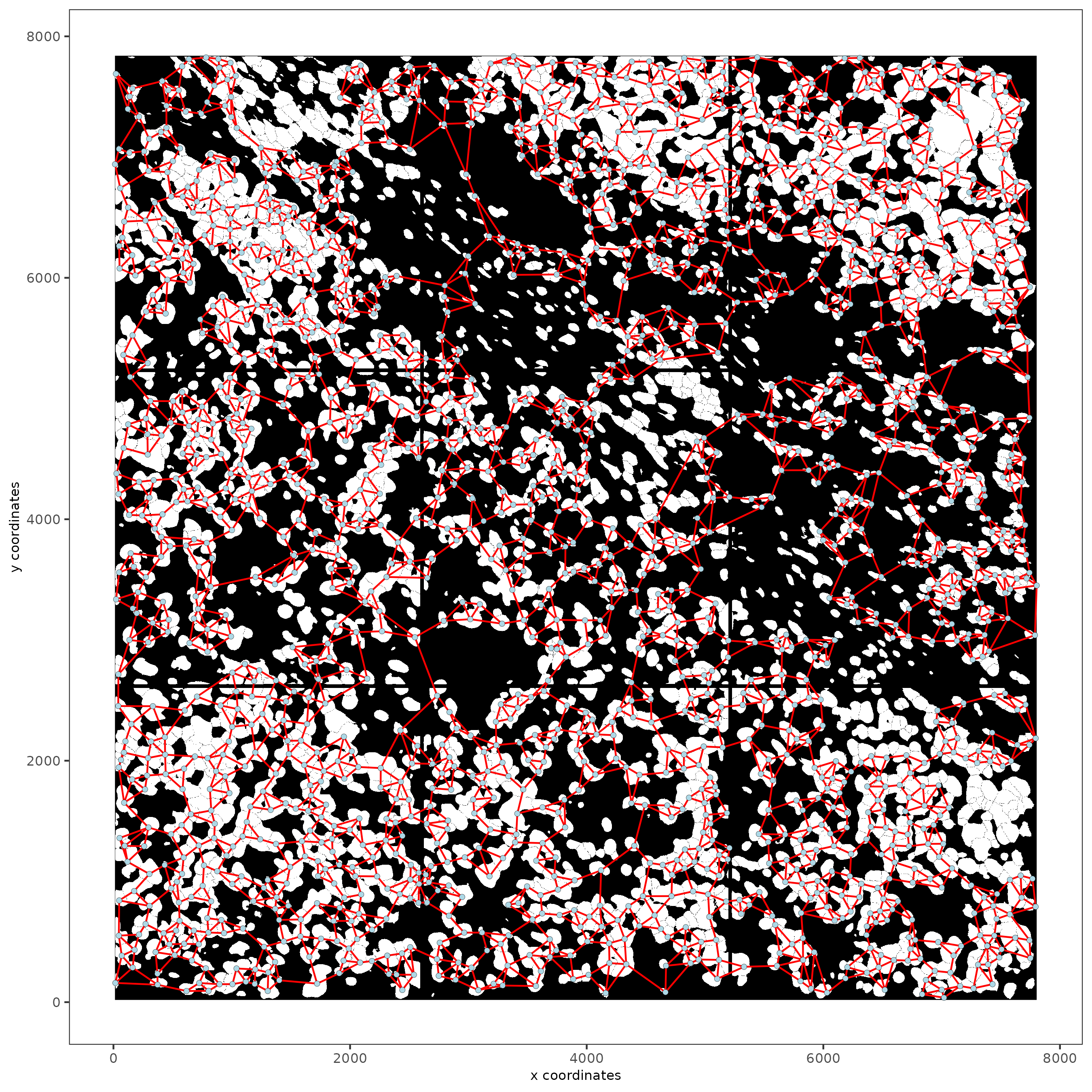
Part 10: Create a Spatial Network#
subc_test = createSpatialNetwork(gobject = subc_test,
                 spat_loc_name = 'cell',
                 minimum_k = 3,
                 maximum_distance_delaunay = 100)

spatPlot2D(gobject = subc_test,
    image_name = 'segmentation', show_image = TRUE,
    point_size = 1.5, show_network = TRUE)
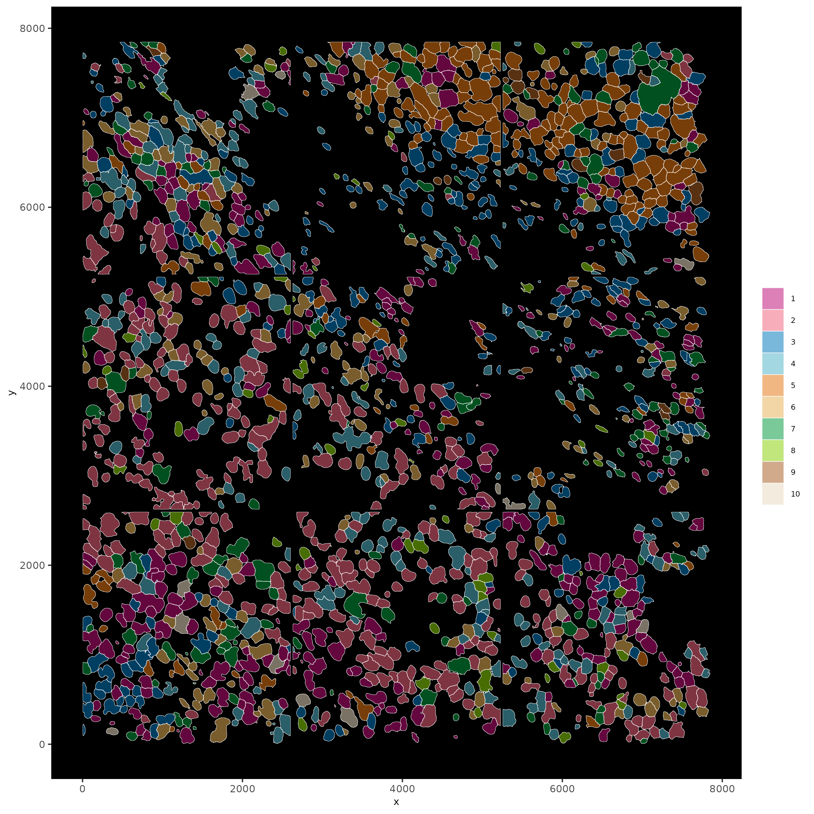
Part 11: Visualize SubCellular Data#
# Visualize clustered cells
spatInSituPlotPoints(subc_test,
            show_polygon = TRUE,
            polygon_feat_type = 'cell',
            polygon_color = 'white',
            polygon_line_size = 0.1,
            polygon_fill = 'leiden_clus',
            polygon_fill_as_factor = T ,
            polygon_fill_code = colorcode)
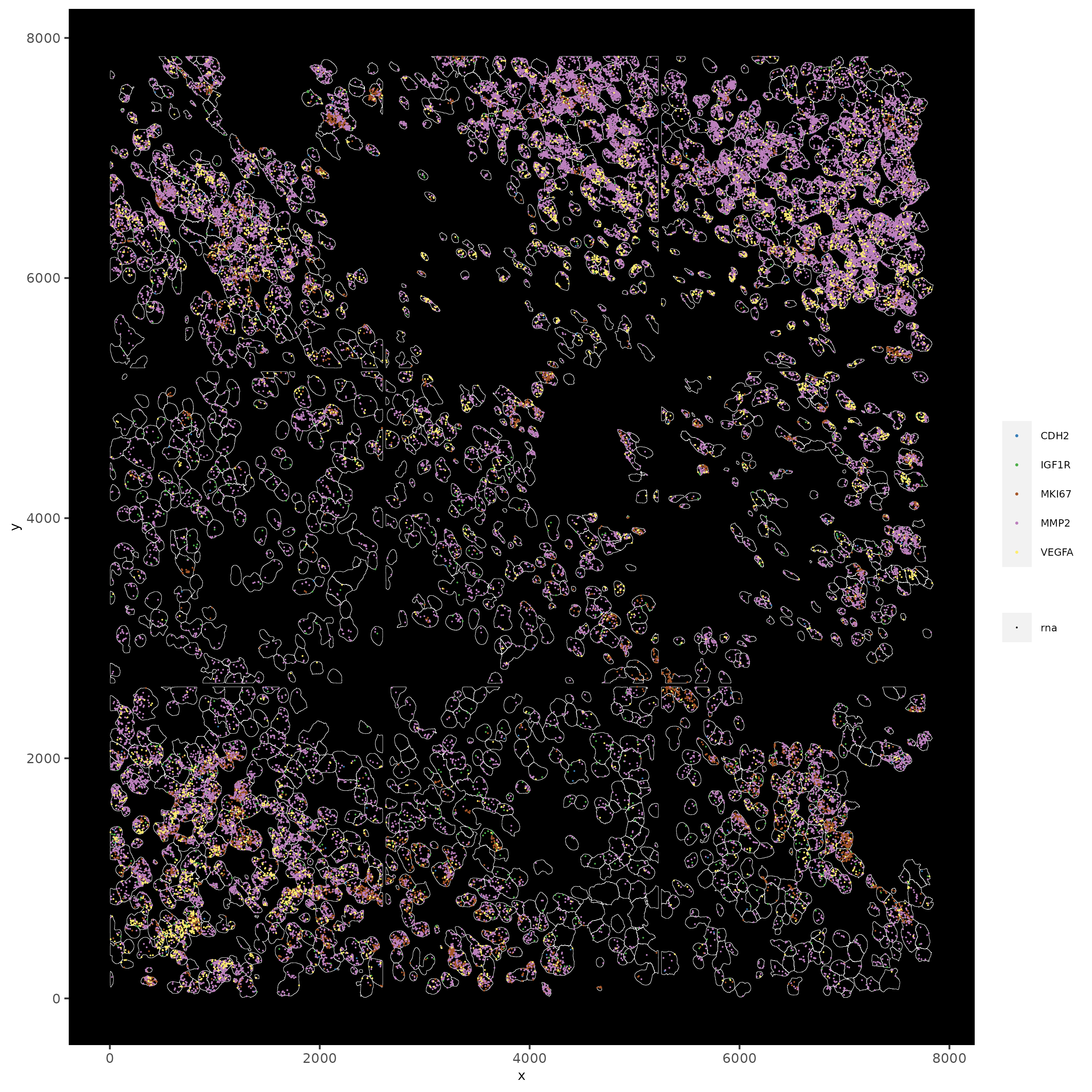
# individual plotting of transcripts and polygon information
# all cells
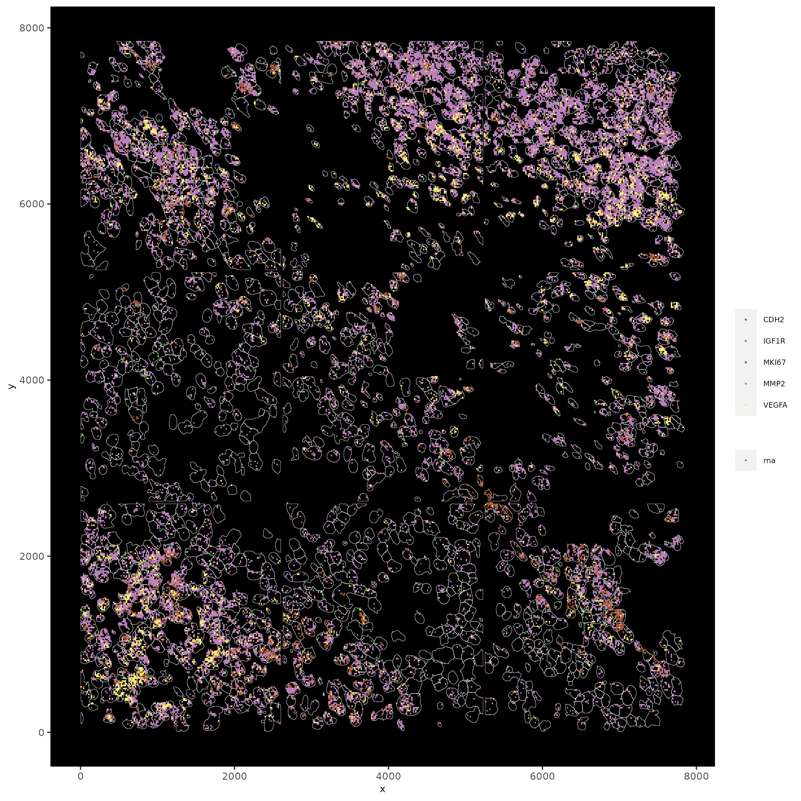
spatInSituPlotPoints(testobj,
feats = list('rna' = c("MMP2", "VEGFA", "IGF1R", 'CDH2', 'MKI67')),
point_size = 0.2,
show_polygon = TRUE,
polygon_feat_type = 'cell',
polygon_color = 'white',
polygon_line_size = 0.1)

# filtered cells
spatInSituPlotPoints(subc_test,
            feats = list('rna' = c("MMP2", "VEGFA", "IGF1R", 'CDH2', 'MKI67')),
            point_size = 0.2,
            show_polygon = TRUE,
            polygon_feat_type = 'cell',
            polygon_color = 'white',
            polygon_line_size = 0.1)
# faster plotting method if you have many points
spatInSituPlotPoints(subc_test,
            plot_method = 'scattermore',
            feats = list('rna' = c("MMP2", "VEGFA", "IGF1R", 'CDH2', 'MKI67')),
            point_size = 0.2,
            show_polygon = TRUE,
            polygon_feat_type = 'cell',
            polygon_color = 'white',
            polygon_line_size = 0.1)
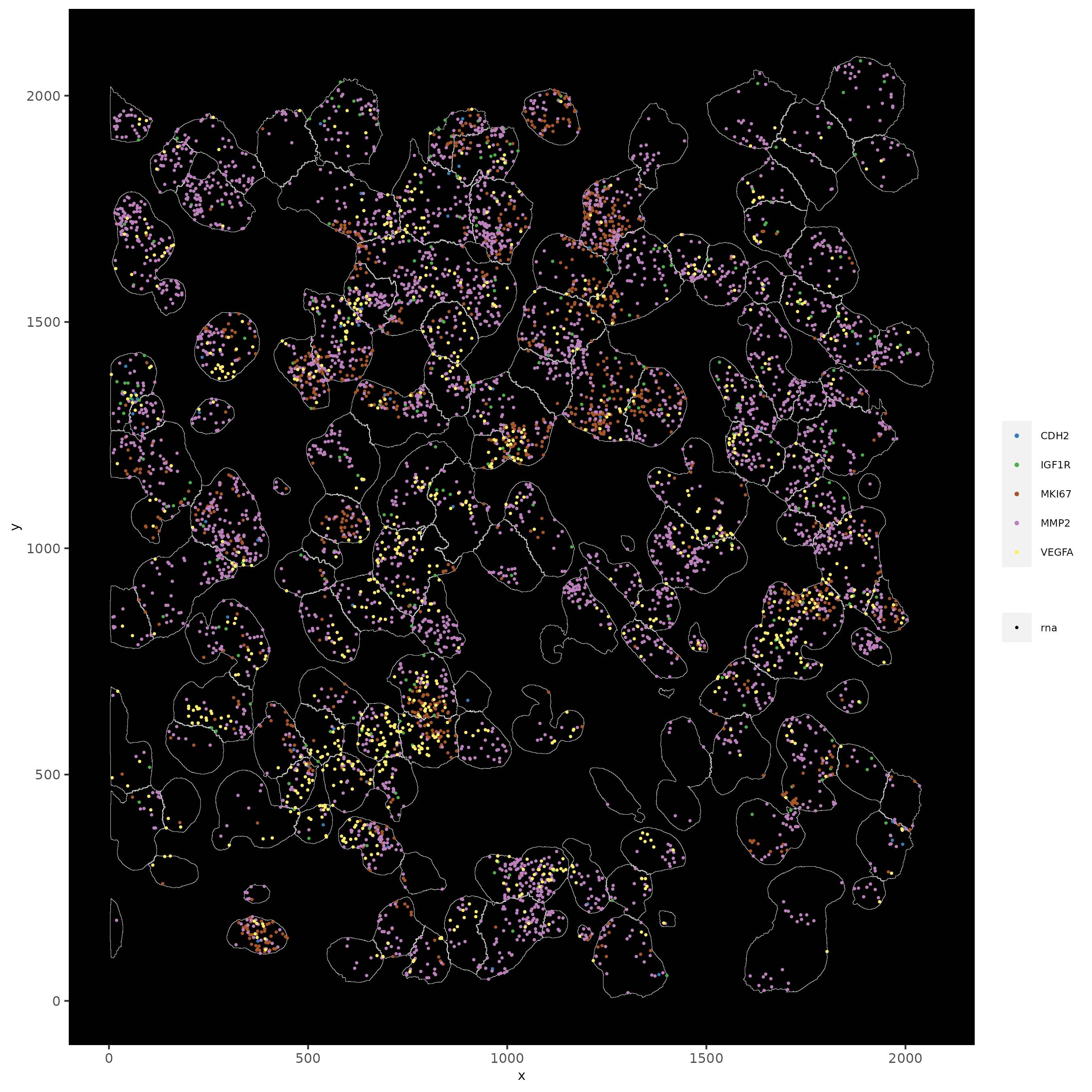
11.1 Subset by Location#
# can be used to focus on specific spatial structures
# to zoom in on niche environments

subloc = subsetGiottoLocs(subc_test,
            x_min = 0, x_max = 2000,
            y_min = 0, y_max = 2000,
            poly_info = 'cell')

# show subset of genes
spatInSituPlotPoints(subloc,
            feats = list('rna' = c("MMP2", "VEGFA", "IGF1R", 'CDH2', 'MKI67')),
            point_size = 0.6,
            show_polygon = TRUE,
            polygon_feat_type = 'cell',
            polygon_color = 'white',
            polygon_line_size = 0.1)
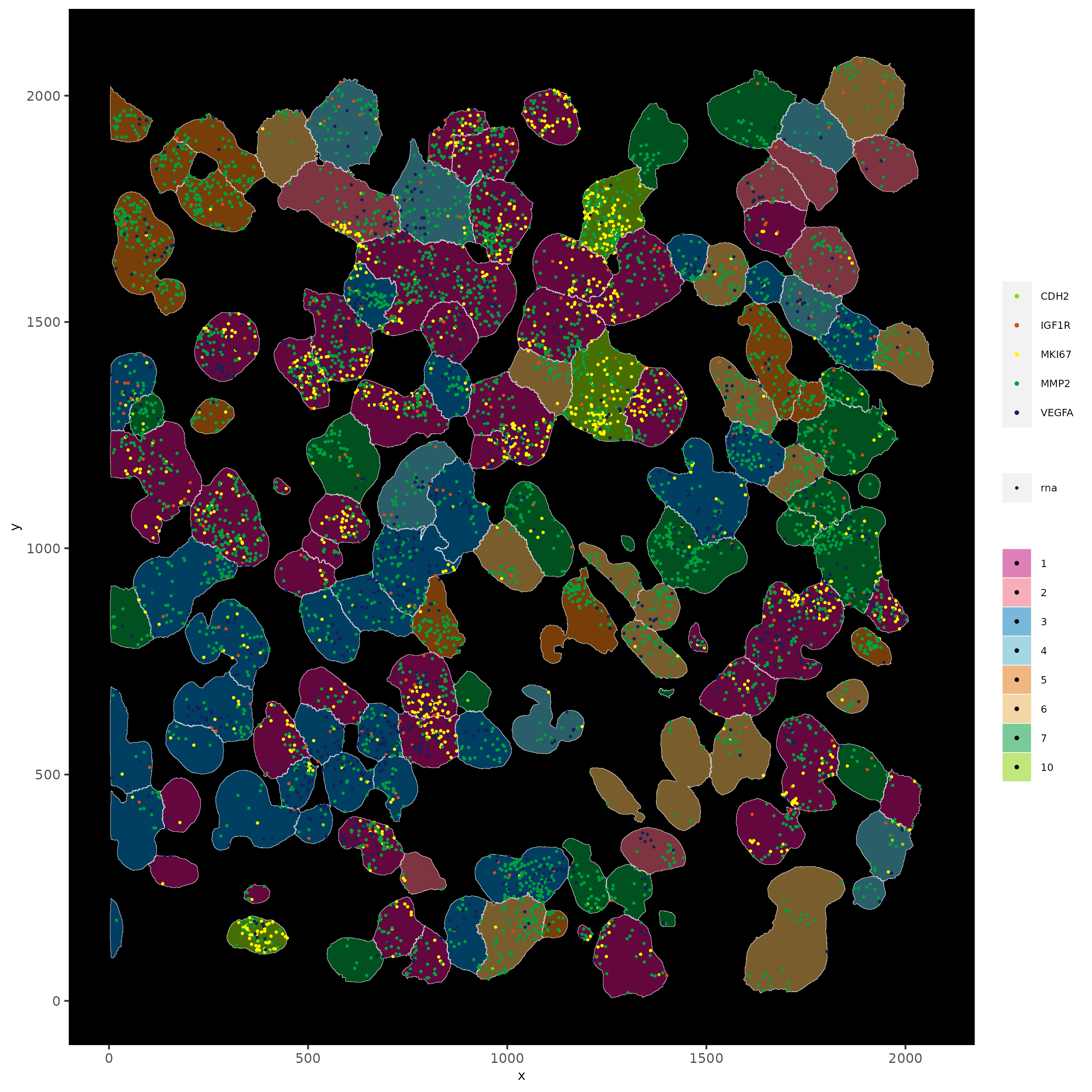
# show subset of genes and color cells according to clusters
spatInSituPlotPoints(subloc,
            feats = list('rna' = c("MMP2", "VEGFA", "IGF1R", 'CDH2', 'MKI67')),
            point_size = 0.6,
            show_polygon = TRUE,
            polygon_feat_type = 'cell',
            polygon_color = 'white',
            polygon_line_size = 0.1,
            polygon_fill = 'leiden_clus',
            polygon_fill_as_factor = T,
            polygon_fill_code = colorcode,
            feats_color_code = featcolor)
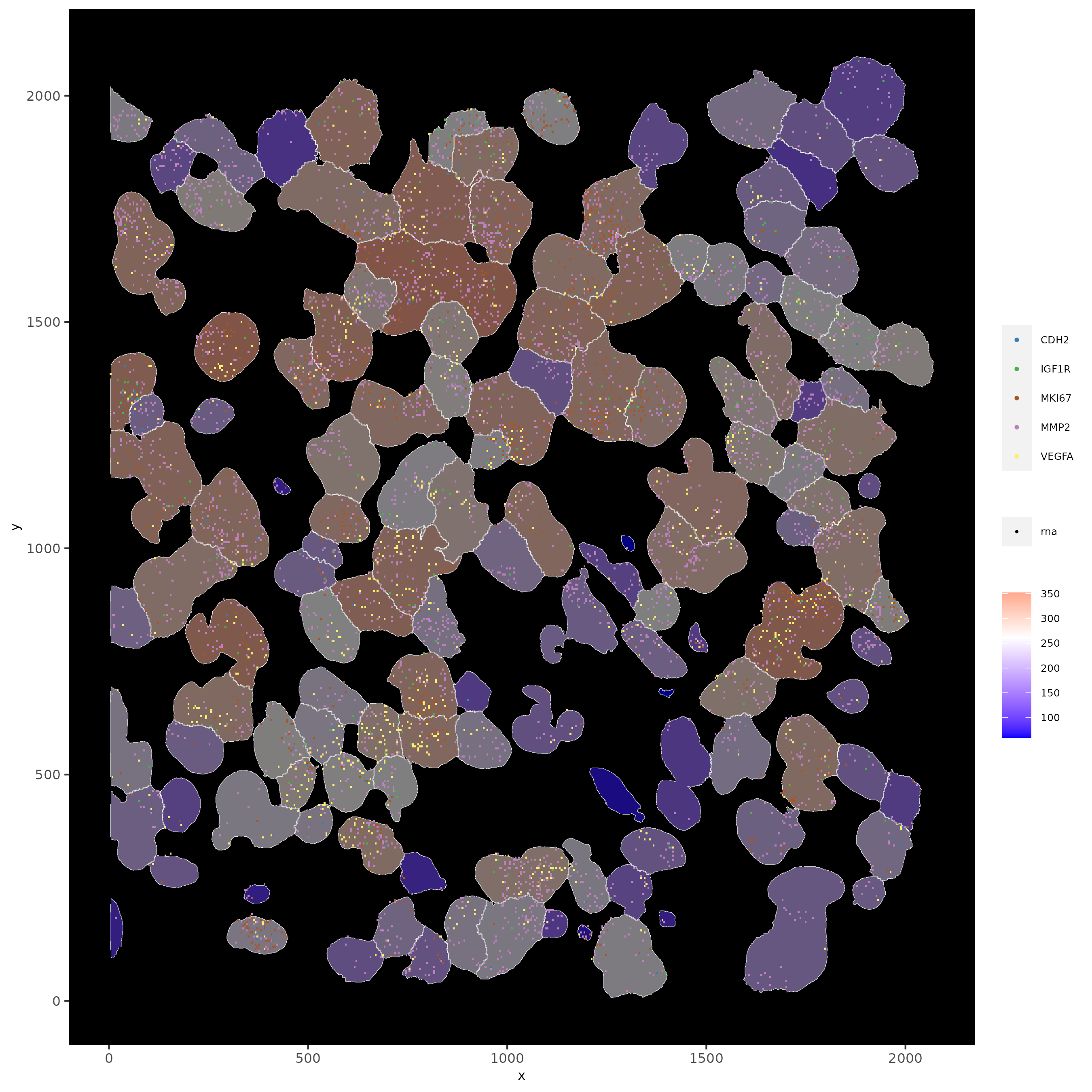
# show subset of genes and color cells according to total expression
# use a faster and more efficient point plotting method = scattermore
spatInSituPlotPoints(subloc,
            plot_method = 'scattermore',
            feats = list('rna' = c("MMP2", "VEGFA", "IGF1R", 'CDH2', 'MKI67')),
            point_size = 0.6,
            show_polygon = TRUE,
            polygon_feat_type = 'cell',
            polygon_color = 'white',
            polygon_line_size = 0.1,
            polygon_fill = 'total_expr',
            polygon_fill_as_factor = F)
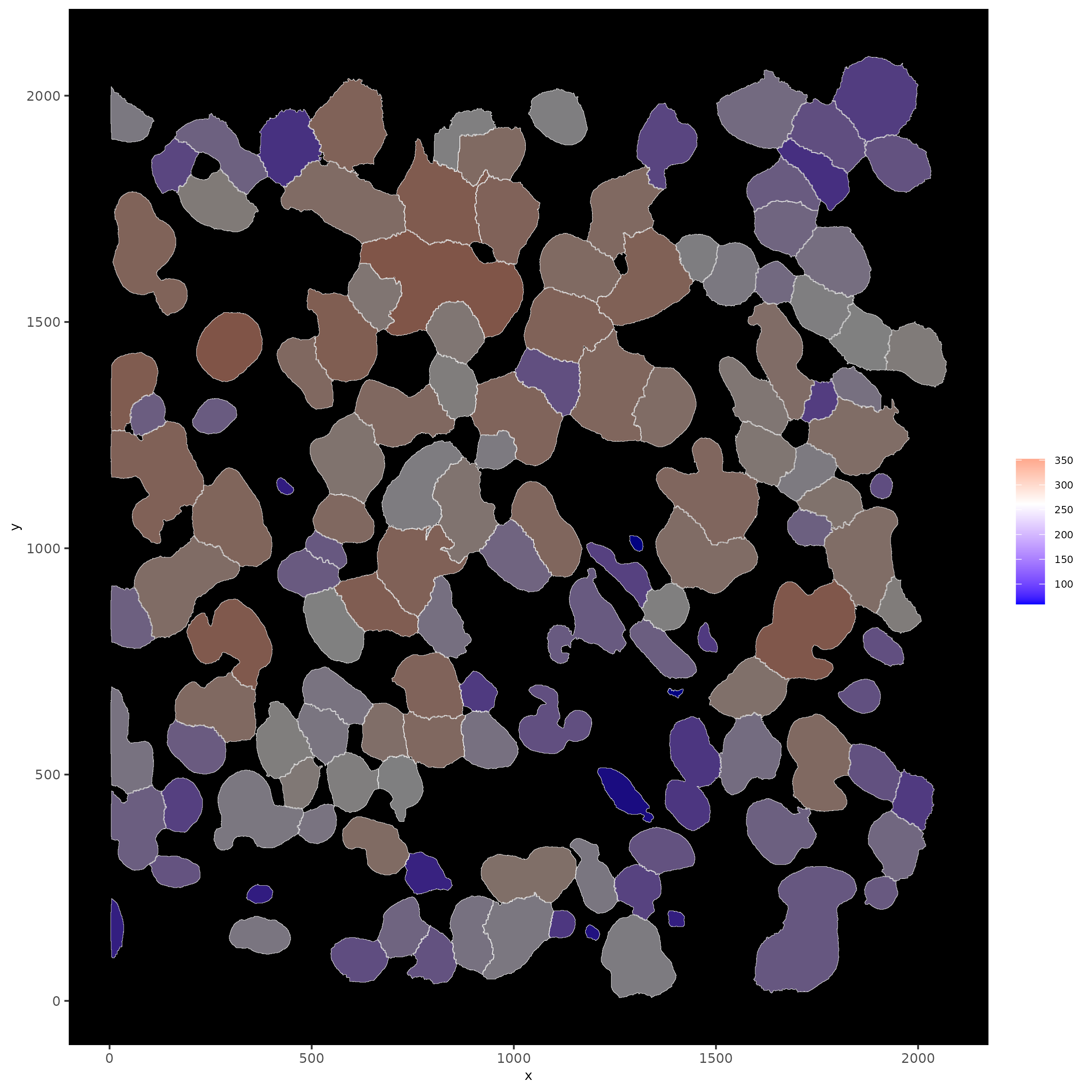
# show cells and color them according to total expression
spatInSituPlotPoints(subloc,
            show_polygon = TRUE,
            polygon_feat_type = 'cell',
            polygon_color = 'white',
            polygon_line_size = 0.1,
            polygon_fill = 'total_expr',
            polygon_fill_as_factor = F)
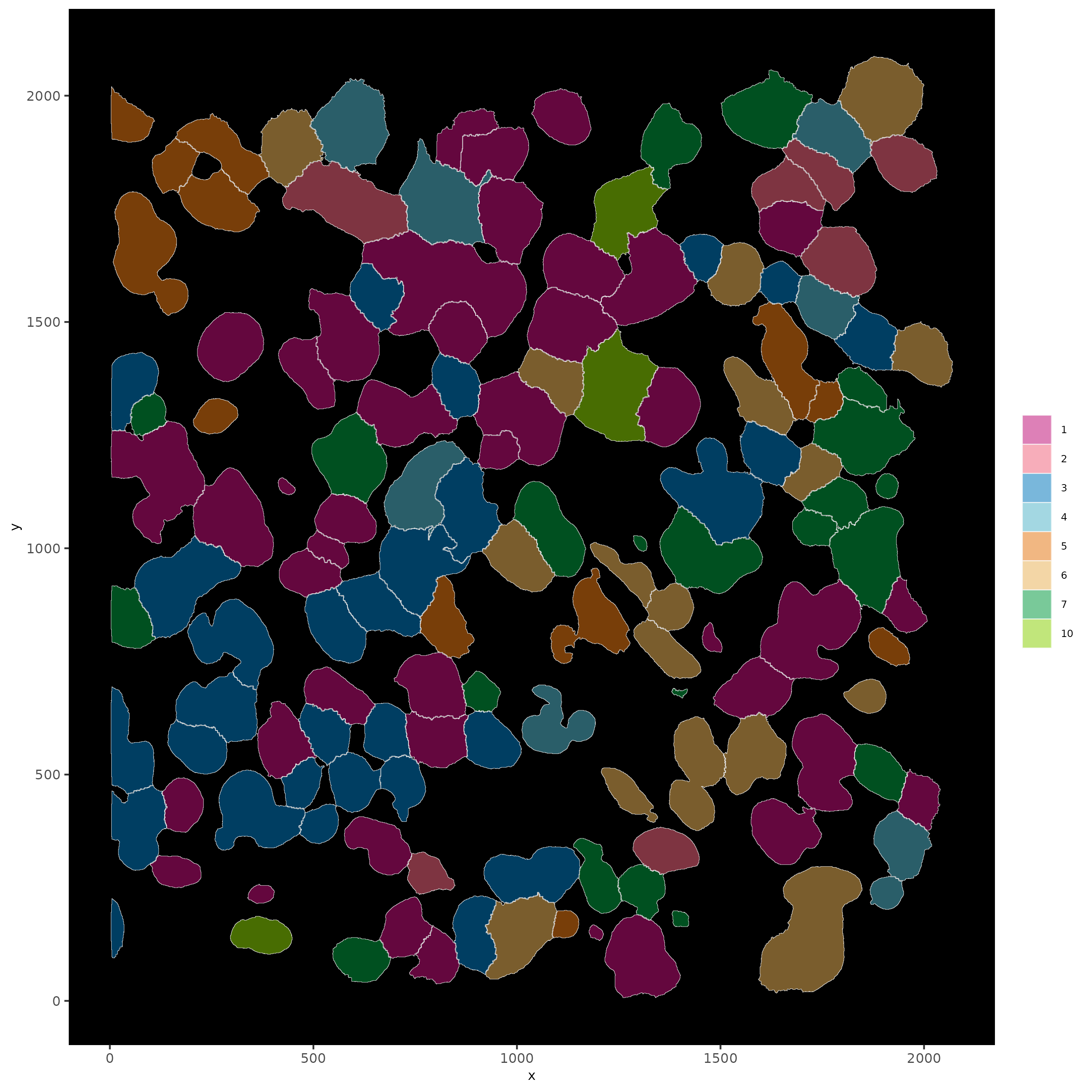
# show cells and color them according to total cluster information
spatInSituPlotPoints(subloc,
            show_polygon = TRUE,
            polygon_feat_type = 'cell',
            polygon_color = 'white',
            polygon_line_size = 0.1,
            polygon_fill = 'leiden_clus',
            polygon_fill_as_factor = T,
            polygon_fill_code = colorcode)
Part 12: Find Interaction Changed Features#
# find interaction changed Features
# In this case, features are genes whose expression difference is associated with a neighboring cell type
future::plan('multisession', workers = 4) # sometimes unstable, restart R session
test = findInteractionChangedFeats(gobject = subc_test,
cluster_column = 'leiden_clus')
test$ICFscores[type_int == 'hetero']
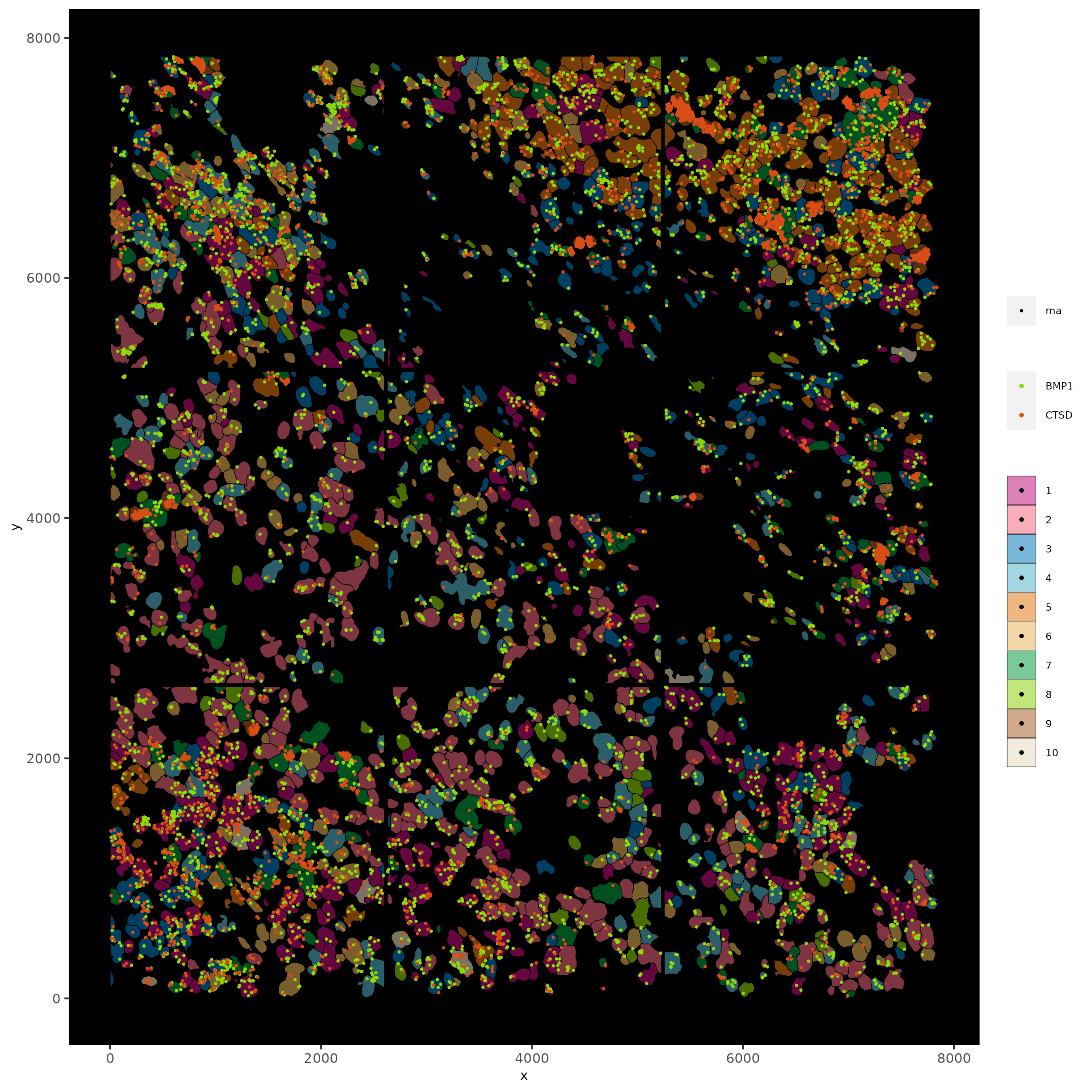
spatInSituPlotPoints(subc_test,
feats = list('rna' = c("CTSD", "BMP1")),
point_size = 0.6,
show_polygon = TRUE,
polygon_feat_type = 'cell',
polygon_color = 'black',
polygon_line_size = 0.1,
polygon_fill = 'leiden_clus',
polygon_fill_as_factor = T,
polygon_fill_code = colorcode,
feats_color_code = featcolor)