Spatial co-expression#
- Date:
4/10/23
1 Dataset explanation#
Here we will use the visium mini dataset, which is a subset of the Visium 10X mouse brain dataset, to illustrate how to perform a spatial co-expression analysis. This mini visium dataset has been fully processed and is easily available through the GiottoData package.
2 Start Giotto#
# Ensure Giotto Suite is installed
if(!"Giotto" %in% installed.packages()) {
  devtools::install_github("drieslab/Giotto@suite")
}
library(Giotto)

# Ensure Giotto Data is installed
if(!"GiottoData" %in% installed.packages()) {
  devtools::install_github("drieslab/GiottoData")
}
library(GiottoData)

# Ensure the Python environment for Giotto has been installed
genv_exists = checkGiottoEnvironment()
if(!genv_exists){
  # The following command need only be run once to install the Giotto environment
  installGiottoEnvironment()
}
3 Load the mini Giotto object#
visium = loadGiottoMini(dataset = 'visium')
1. read Giotto object
2. read Giotto feature information
3. read Giotto spatial information
4. read Giotto image information
no external python path was provided, but a giotto python environment was found
 and will be used

no external python path was provided, but a giotto python environment was found
 and will be used
4 Calculate spatially variable genes#
make sure that you have already created a spatial network
you can identify spatial genes with any type of method, here we will use the binSpect method
showGiottoSpatNetworks(visium)
└──Spatial unit "cell"
   ├──S4 spatialNetworkObj "Delaunay_network"   (1770 rows)
   │                      from                 to sdimx_begin sdimy_begin sdimx_end
   │     1: AAAGGGATGTAGCAAG-1 TCAAACAACCGCGTCG-1        5477       -4125      5340
   │     2: AAAGGGATGTAGCAAG-1 ACGATCATACATAGAG-1        5477       -4125      5546
   │     3: AAAGGGATGTAGCAAG-1 TATGCTCCCTACTTAC-1        5477       -4125      5408
   │     4: AAAGGGATGTAGCAAG-1 TTGTTCAGTGTGCTAC-1        5477       -4125      5615
   │        sdimy_end distance      weight
   │     1:     -4125 137.0000 0.007299270
   │     2:     -4244 137.5573 0.007269700
   │     3:     -4244 137.5573 0.007269700
   │     4:     -4125 138.0000 0.007246377
   │
   └──S4 spatialNetworkObj "spatial_network"   (3288 rows)
                          from                 to sdimx_begin sdimy_begin sdimx_end
         1: AAAGGGATGTAGCAAG-1 TCAAACAACCGCGTCG-1        5477       -4125      5340
         2: AAAGGGATGTAGCAAG-1 ACGATCATACATAGAG-1        5477       -4125      5546
         3: AAAGGGATGTAGCAAG-1 TATGCTCCCTACTTAC-1        5477       -4125      5408
         4: AAAGGGATGTAGCAAG-1 TTGTTCAGTGTGCTAC-1        5477       -4125      5615
            sdimy_end distance      weight
         1:     -4125 137.0000 0.007246377
         2:     -4244 137.5573 0.007217233
         3:     -4244 137.5573 0.007217233
         4:     -4125 138.0000 0.007194245
ranktest = binSpect(visium, bin_method = 'rank',
                    calc_hub = T, hub_min_int = 5,
                    spatial_network_name = 'Delaunay_network')
This is the single parameter version of binSpect
1. matrix binarization complete

2. spatial enrichment test completed

3. (optional) average expression of high expressing cells calculated

4. (optional) number of high expressing cells calculated
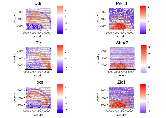
spatFeatPlot2D(visium,
               expression_values = 'scaled',
               feats = ranktest$feats[1:6], cow_n_col = 2, point_size = 1.5)
5 Identify spatially correlated genes#
here we will subset on the top 300 spatial genes identified with binSpect.
we will also show how to identify the top spatially correlated genes with a gene of interest
# 3.1 cluster the top 500 spatial genes into 20 clusters
ext_spatial_genes = ranktest[1:300,]$feats
# here we use existing detectSpatialCorGenes function to calculate pairwise distances between genes (but set network_smoothing=0 to use default clustering)
spat_cor_netw_DT = detectSpatialCorFeats(visium,
method = 'network',
spatial_network_name = 'spatial_network',
subset_feats = ext_spatial_genes)
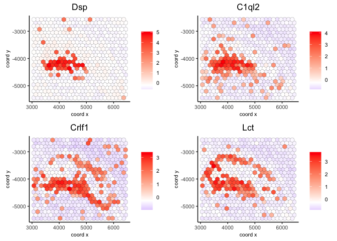
# 3.2 identify most similar spatially correlated genes for one gene
top10_genes = showSpatialCorFeats(spat_cor_netw_DT, feats = 'Dsp', show_top_feats = 10)
spatFeatPlot2D(visium,
expression_values = 'scaled',
feats = top10_genes$variable[1:4], point_size = 3)
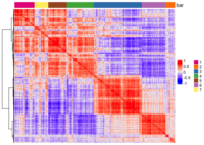
6 Cluster and visualize spatially correlated genes#
use the heatmap to identify spatial co-expression modules and adjust the number of clusters (k) accordingly
# 3.3 identify potenial spatial co-expression
spat_cor_netw_DT = clusterSpatialCorFeats(spat_cor_netw_DT, name = 'spat_netw_clus', k = 7)

# visualize clusters
heatmSpatialCorFeats(visium,
                     spatCorObject = spat_cor_netw_DT,
                     use_clus_name = 'spat_netw_clus',
                     heatmap_legend_param = list(title = NULL),
                     save_param = list(base_height = 6, base_width = 8, units = 'cm'))
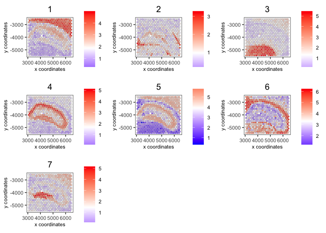
7 Create metagenes/co-expression modules and visualize#
extract a balanced set of genes from each co-expression module.
aggregate genes into metagenes.
# 3.4 create metagenes / co-expression modules
cluster_genes = getBalancedSpatCoexpressionFeats(spat_cor_netw_DT, maximum = 30)
[1] 1
[1] 2
There are only 19 features for cluster 2
 Maximum will be set to 19
[1] 3
[1] 4
[1] 5
[1] 6
[1] 7
There are only 25 features for cluster 7
 Maximum will be set to 25
visium = createMetafeats(visium, feat_clusters = cluster_genes, name = 'cluster_metagene')
cluster_metagene has already been used, will be overwritten
> " cluster_metagene " already exists and will be replaced with new spatial
 enrichment results
spatCellPlot(visium,
             spat_enr_names = 'cluster_metagene',
             cell_annotation_values = as.character(c(1:7)),
             point_size = 1, cow_n_col = 3)
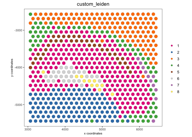
8 (optional) Spatially informed clustering#
Here we illustrate how to use information from #5 as input for clustering using the standard pipeline (PCA > nearest-neighbors > leiden clusters).
my_spatial_genes = names(cluster_genes)

visium <- runPCA(gobject = visium,
                      feats_to_use = my_spatial_genes,
                      name = 'custom_pca')
a custom vector of genes will be used to subset the matrix
class of selected matrix: dgCMatrix
Warning in (function (A, nv = 5, nu = nv, maxit = 1000, work = nv + 7, reorth =
TRUE, : You're computing too large a percentage of total singular values, use a
standard svd instead.
custom_pca has already been used, will be overwritten
> custom_pca already exists and will be replaced with new dimension reduction
 object
visium <- runUMAP(visium,
                       dim_reduction_name = 'custom_pca',
                       dimensions_to_use = 1:20,
                       name = 'custom_umap')
custom_umap has already been used, will be overwritten
> custom_umap already exists and will be replaced with new dimension reduction
 object
visium <- createNearestNetwork(gobject = visium,
                                    dim_reduction_name = 'custom_pca',
                                    dimensions_to_use = 1:20, k = 5,
                                    name = 'custom_NN')
IGRAPH dbea2e8 DNW- 624 1872 --
+ attr: name (v/c), weight (e/n), distance (e/n), shared (e/n), rank
| (e/n)
+ edges from dbea2e8 (vertex names):
 [1] AAAGGGATGTAGCAAG-1->AACTGGGTCCCGACGT-1
 [2] AAAGGGATGTAGCAAG-1->CAGCTCGTGCTTGTGT-1
 [3] AAAGGGATGTAGCAAG-1->CGTACCTGATAGGCCT-1
 [4] AAATGGCATGTCTTGT-1->GTGCACGAAAGTGACT-1
 [5] AAATGGCATGTCTTGT-1->CTCTGCGAAGCAAGCA-1
 [6] AAATGGCATGTCTTGT-1->GATATCTCATGCAATA-1
 [7] AAATGGTCAATGTGCC-1->CGAAGTTGCTCTGTGT-1
+ ... omitted several edges
> " custom_NN " already exists and will be replaced with new nearest neighbor
 network
visium <- doLeidenCluster(gobject = visium,
                               network_name = 'custom_NN',
                               resolution = 0.15, n_iterations = 1000,
                               name = 'custom_leiden')
custom_leiden has already been used, will be overwritten
spatPlot2D(visium,
           cell_color = 'custom_leiden', point_size = 4)
9 Session Info#
sessionInfo()
R version 4.2.2 (2022-10-31)
Platform: aarch64-apple-darwin20 (64-bit)
Running under: macOS Ventura 13.2.1

Matrix products: default
BLAS:   /Library/Frameworks/R.framework/Versions/4.2-arm64/Resources/lib/libRblas.0.dylib
LAPACK: /Library/Frameworks/R.framework/Versions/4.2-arm64/Resources/lib/libRlapack.dylib

locale:
[1] en_US.UTF-8/en_US.UTF-8/en_US.UTF-8/C/en_US.UTF-8/en_US.UTF-8

attached base packages:
[1] stats     graphics  grDevices utils     datasets  methods   base

other attached packages:
[1] GiottoData_0.2.1 Giotto_3.2.1

loaded via a namespace (and not attached):
 [1] rsvd_1.0.5            Rcpp_1.0.10           here_1.0.1
 [4] lattice_0.20-45       circlize_0.4.15       FNN_1.1.3.1
 [7] png_0.1-8             rprojroot_2.0.3       digest_0.6.31
[10] foreach_1.5.2         utf8_1.2.3            R6_2.5.1
[13] stats4_4.2.2          evaluate_0.20         ggplot2_3.4.1
[16] pillar_1.8.1          GlobalOptions_0.1.2   zlibbioc_1.44.0
[19] rlang_1.0.6           irlba_2.3.5.1         rstudioapi_0.14
[22] data.table_1.14.8     magick_2.7.3          S4Vectors_0.36.1
[25] GetoptLong_1.0.5      Matrix_1.5-3          reticulate_1.28
[28] rmarkdown_2.20        labeling_0.4.2        BiocParallel_1.32.5
[31] uwot_0.1.14           beachmat_2.14.0       igraph_1.4.0
[34] munsell_0.5.0         DelayedArray_0.24.0   BiocSingular_1.14.0
[37] compiler_4.2.2        xfun_0.37             pkgconfig_2.0.3
[40] BiocGenerics_0.44.0   shape_1.4.6           htmltools_0.5.4
[43] tidyselect_1.2.0      tibble_3.1.8          IRanges_2.32.0
[46] codetools_0.2-19      matrixStats_0.63.0    fansi_1.0.4
[49] crayon_1.5.2          dplyr_1.1.0           withr_2.5.0
[52] grid_4.2.2            jsonlite_1.8.4        gtable_0.3.1
[55] lifecycle_1.0.3       magrittr_2.0.3        scales_1.2.1
[58] ScaledMatrix_1.6.0    cli_3.6.0             dbscan_1.1-11
[61] farver_2.1.1          XVector_0.38.0        doParallel_1.0.17
[64] generics_0.1.3        vctrs_0.5.2           cowplot_1.1.1
[67] rjson_0.2.21          RColorBrewer_1.1-3    iterators_1.0.14
[70] tools_4.2.2           Biobase_2.58.0        glue_1.6.2
[73] MatrixGenerics_1.10.0 parallel_4.2.2        fastmap_1.1.0
[76] yaml_2.3.7            clue_0.3-64           colorspace_2.1-0
[79] terra_1.7-18          cluster_2.1.4         ComplexHeatmap_2.14.0
[82] knitr_1.42