Mouse Visium Kidney

Date:

2021-08-30

#> Warning: This tutorial was written with Giotto version 2.0.0.9046, your version
#> is 2.0.0.998.This is an older version and results could be slightly different

# Ensure Giotto Suite is installed.
if(!"Giotto" %in% installed.packages()) {
  devtools::install_github("drieslab/Giotto@suite")
}

# Ensure GiottoData, a small, helper module for tutorials, is installed.
if(!"GiottoData" %in% installed.packages()) {
  devtools::install_github("drieslab/GiottoData")
}
# Ensure the Python environment for Giotto has been installed.
library(Giotto)
genv_exists = checkGiottoEnvironment()
if(!genv_exists){
  # The following command need only be run once to install the Giotto environment.
  installGiottoEnvironment()
}

library(GiottoData)

# 1. set working directory
results_folder = '/path/to/directory/'

# Optional: Specify a path to a Python executable within a conda or miniconda
# environment. If set to NULL (default), the Python executable within the previously
# installed Giotto environment will be used.
python_path = NULL # alternatively, "/local/python/path/python" if desired.

Dataset explanation

10X genomics recently launched a new platform to obtain spatial expression data using a Visium Spatial Gene Expression slide.

The Visium kidney data to run this tutorial can be found here

Visium technology:

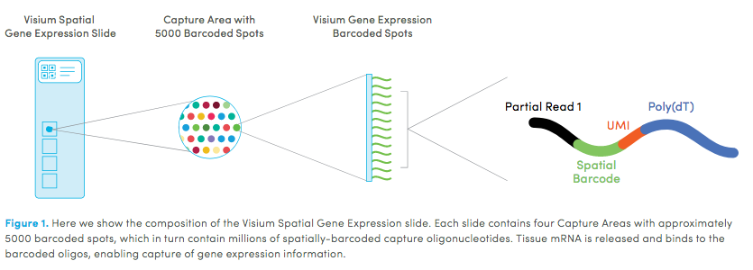
High resolution png from original tissue:

Part 1: Giotto global instructions and preparations

## create instructions
instrs = createGiottoInstructions(save_dir = results_folder,
                                  save_plot = TRUE,
                                  show_plot = FALSE,
                                  python_path = python_path)

## provide path to visium folder
data_path = '/path/to/Kidney_data/'

part 2: Create Giotto object & process data

## directly from visium folder
visium_kidney = createGiottoVisiumObject(visium_dir = data_path,
                                         expr_data = 'raw',
                                         png_name = 'tissue_lowres_image.png',
                                         gene_column_index = 2,
                                         instructions = instrs)

## check metadata
pDataDT(visium_kidney)

# check available image names
showGiottoImageNames(visium_kidney) # "image" is the default name

## show aligned image
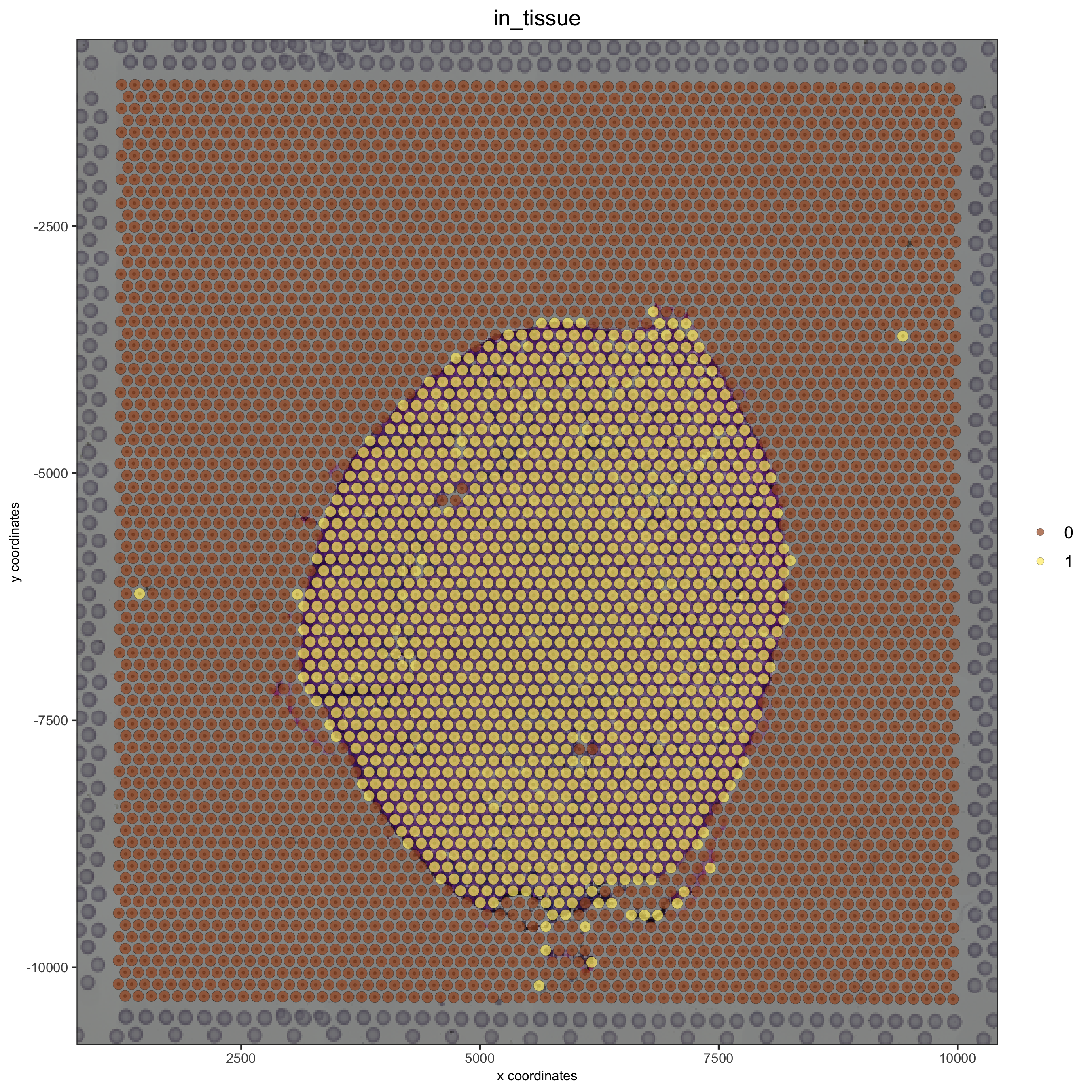
spatPlot(gobject = visium_kidney, cell_color = 'in_tissue', show_image = T, point_alpha = 0.7)

## subset on spots that were covered by tissue
metadata = pDataDT(visium_kidney)
in_tissue_barcodes = metadata[in_tissue == 1]$cell_ID
visium_kidney = subsetGiotto(visium_kidney, cell_ids = in_tissue_barcodes)

## filter
visium_kidney <- filterGiotto(gobject = visium_kidney,
                              expression_threshold = 1,
                              feat_det_in_min_cells = 50,
                              min_det_feats_per_cell = 1000,
                              expression_values = c('raw'),
                              verbose = T)

## normalize
visium_kidney <- normalizeGiotto(gobject = visium_kidney, scalefactor = 6000, verbose = T)

## add gene & cell statistics
visium_kidney <- addStatistics(gobject = visium_kidney)

## visualize
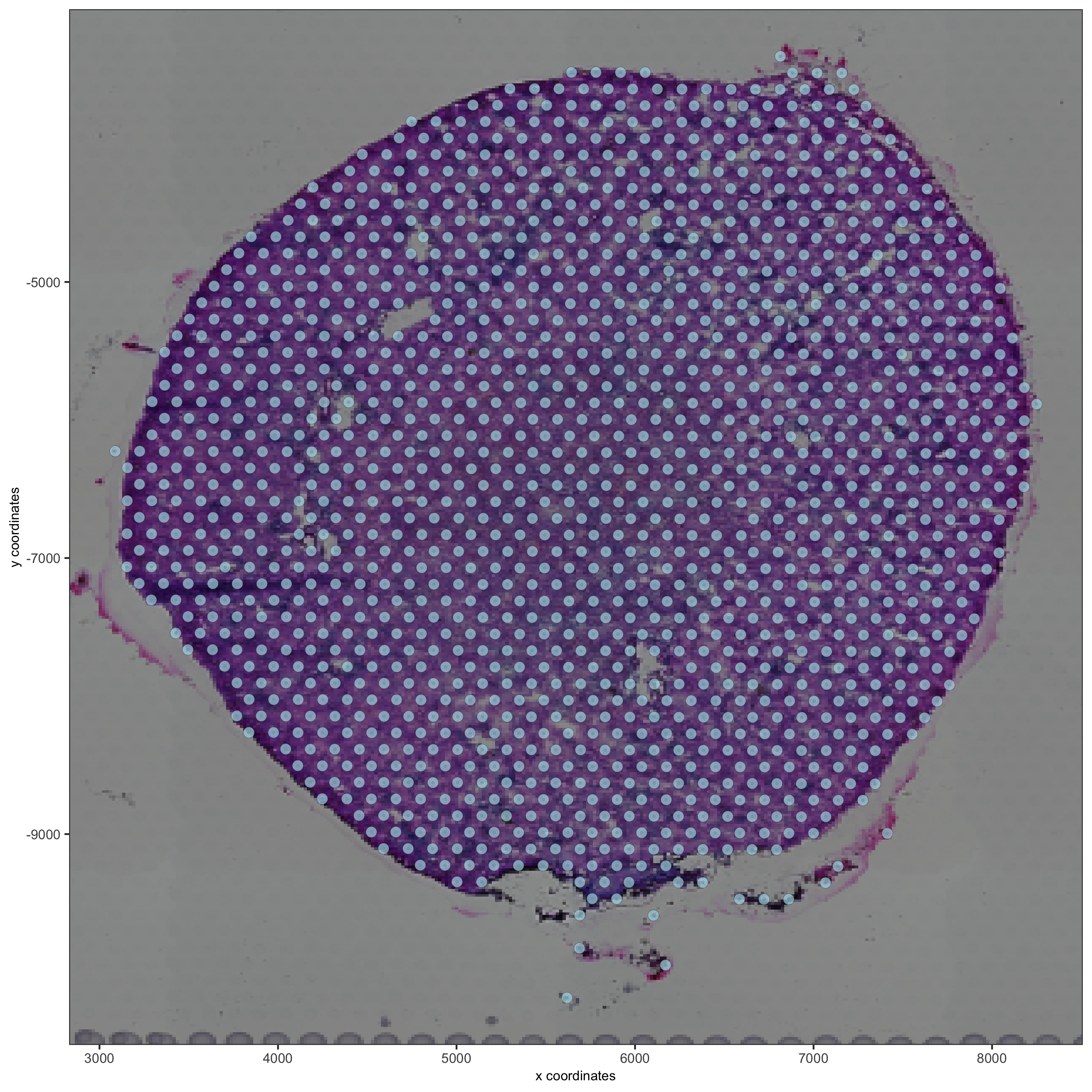
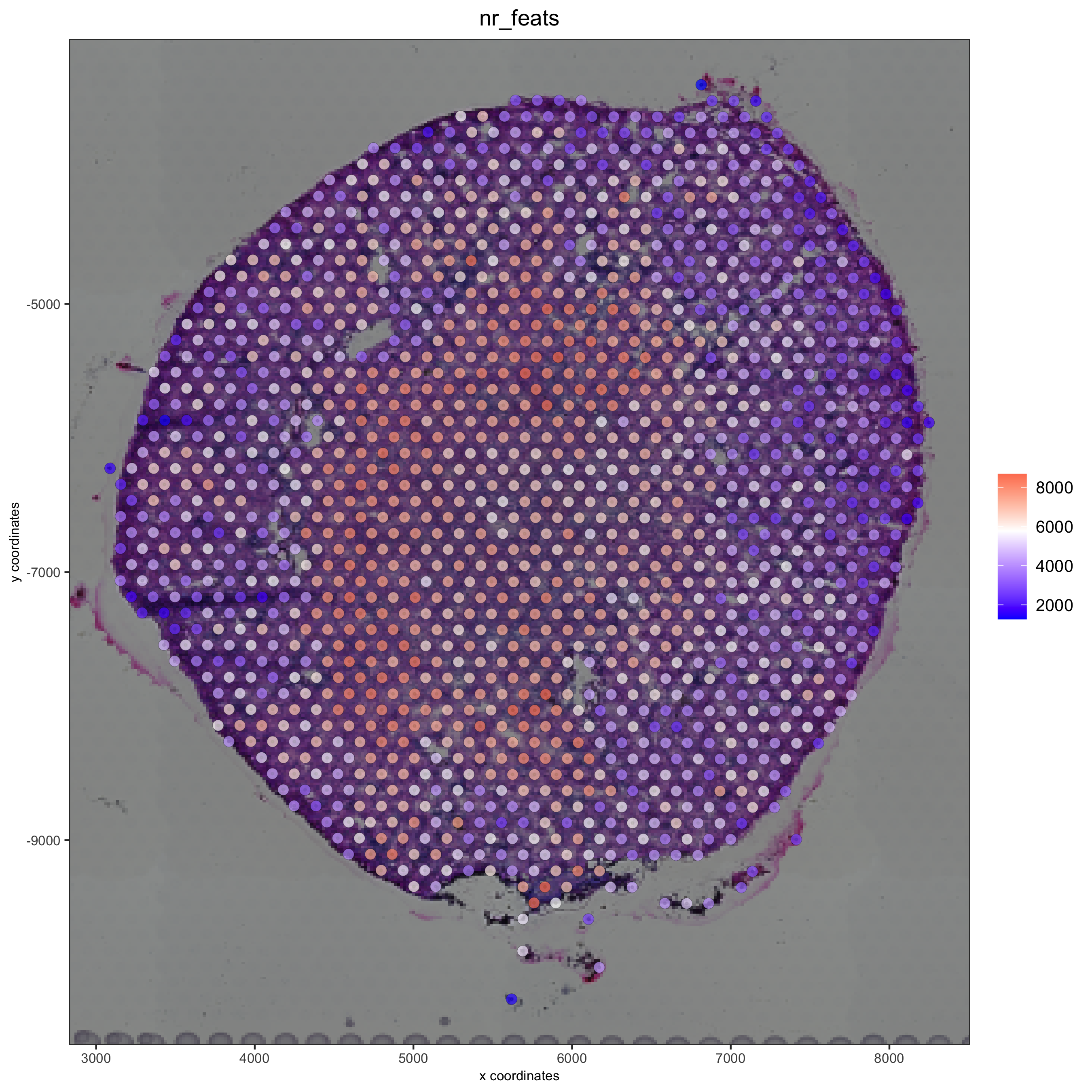
spatPlot2D(gobject = visium_kidney, show_image = T, point_alpha = 0.7)

spatPlot2D(gobject = visium_kidney, show_image = T, point_alpha = 0.7,
           cell_color = 'nr_feats', color_as_factor = F)

part 3: dimension reduction

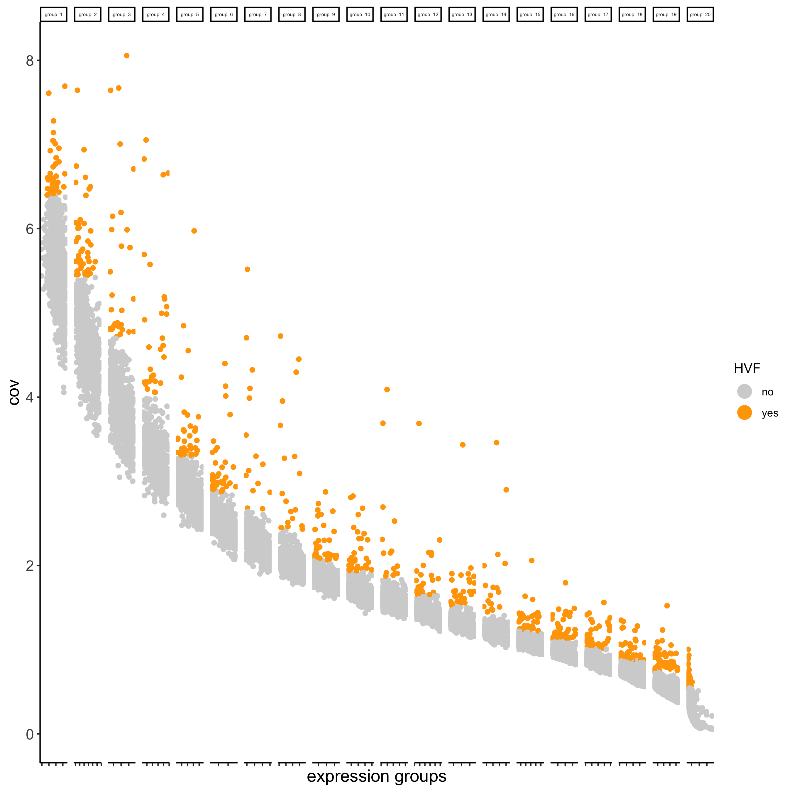
## highly variable features (genes)
visium_kidney <- calculateHVF(gobject = visium_kidney)

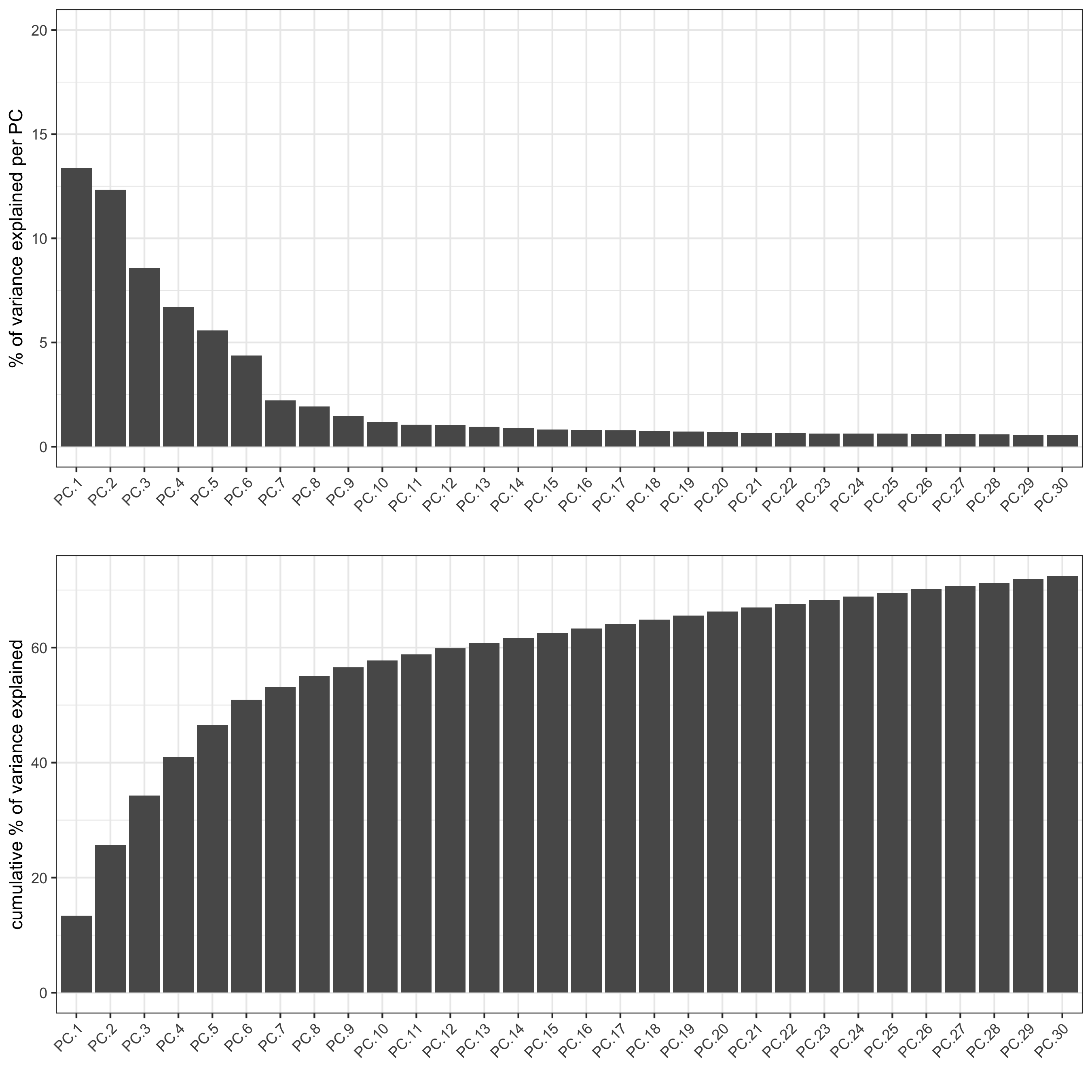
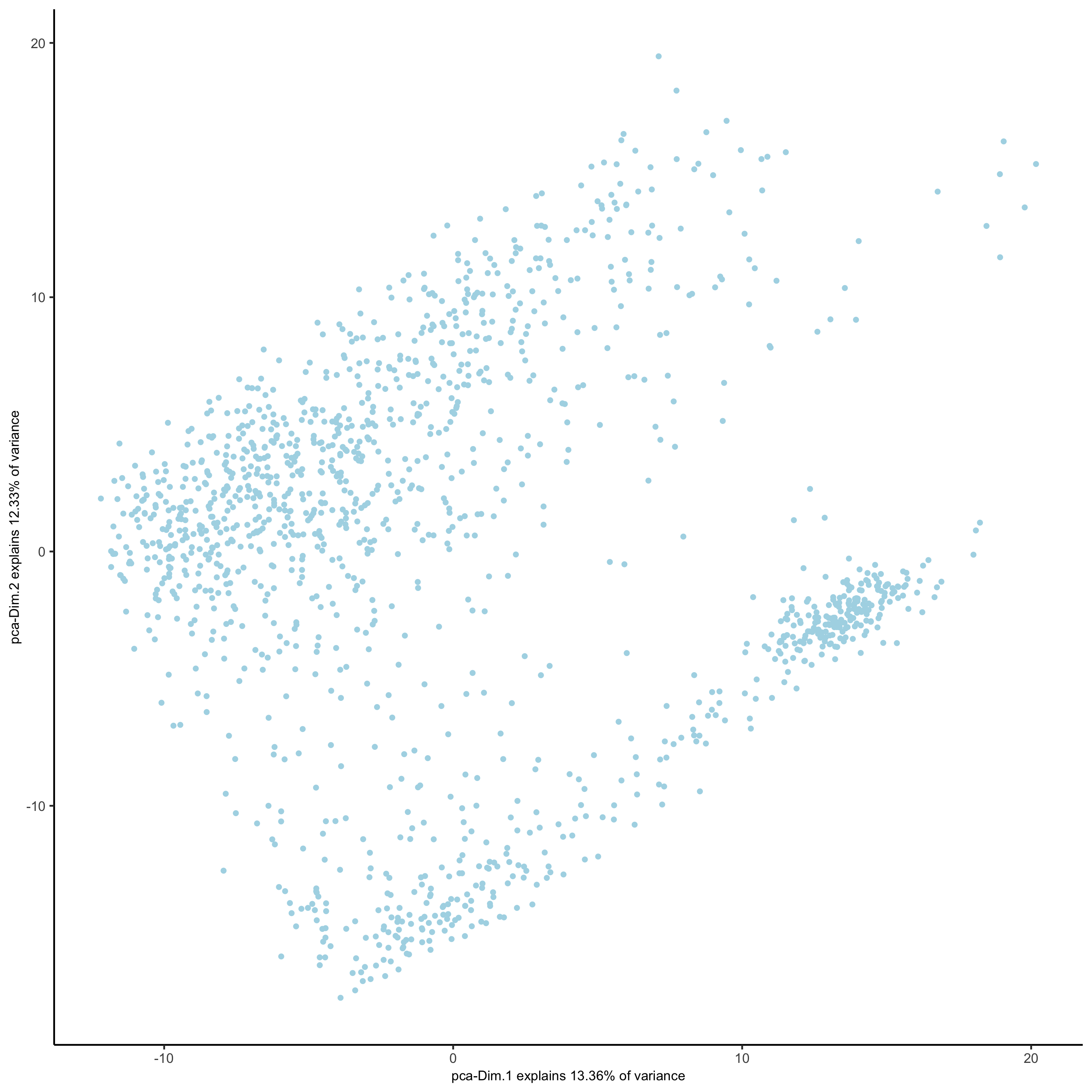
## run PCA on expression values (default)
visium_kidney <- runPCA(gobject = visium_kidney)
screePlot(visium_kidney, ncp = 30)

plotPCA(gobject = visium_kidney)

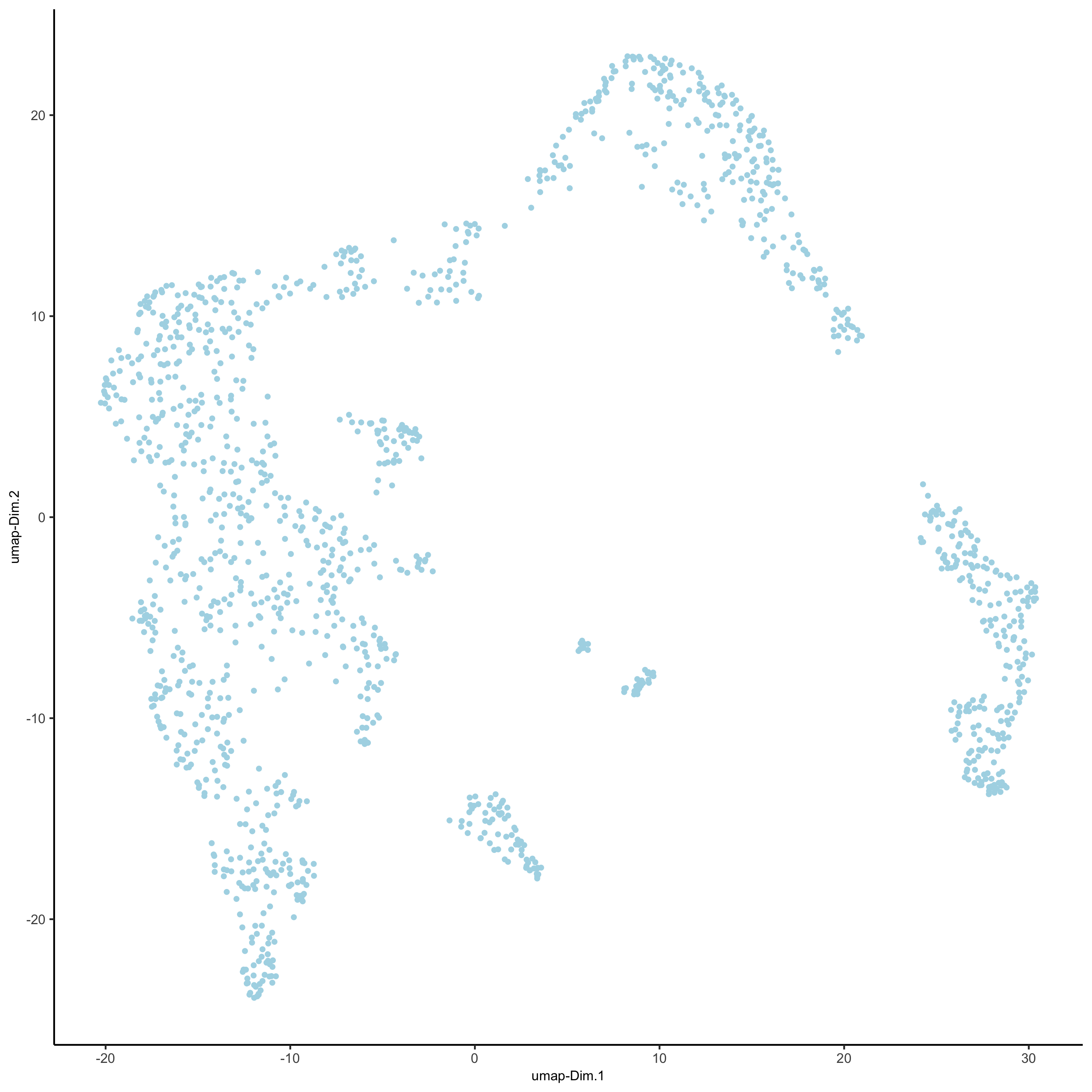
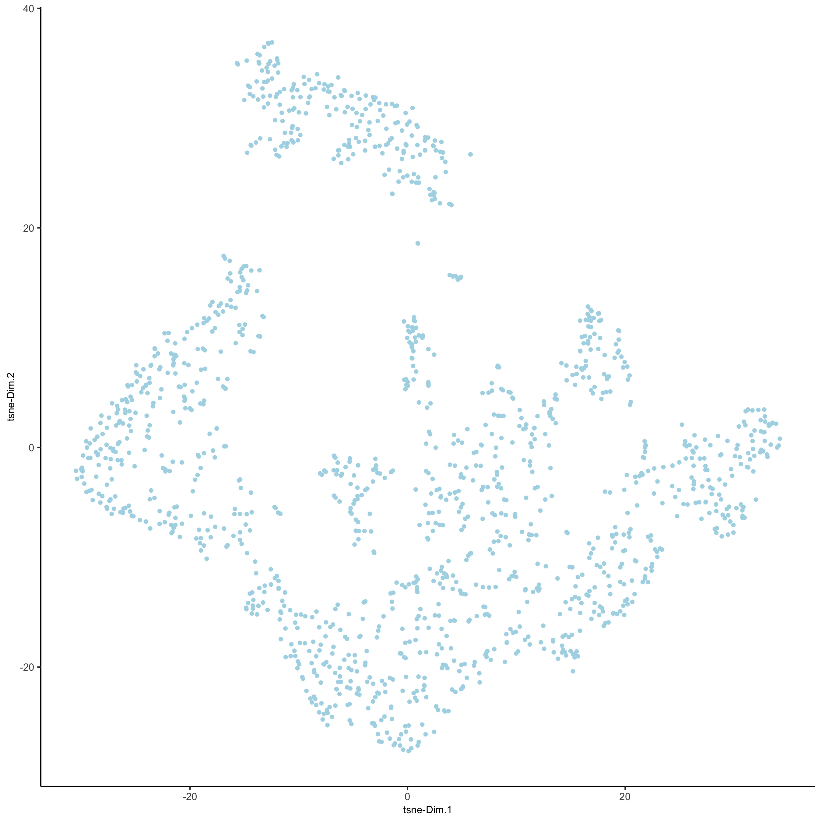
## run UMAP and tSNE on PCA space (default)
visium_kidney <- runUMAP(visium_kidney, dimensions_to_use = 1:10)
plotUMAP(gobject = visium_kidney)

visium_kidney <- runtSNE(visium_kidney, dimensions_to_use = 1:10)
plotTSNE(gobject = visium_kidney)

part 4: cluster

## sNN network (default)
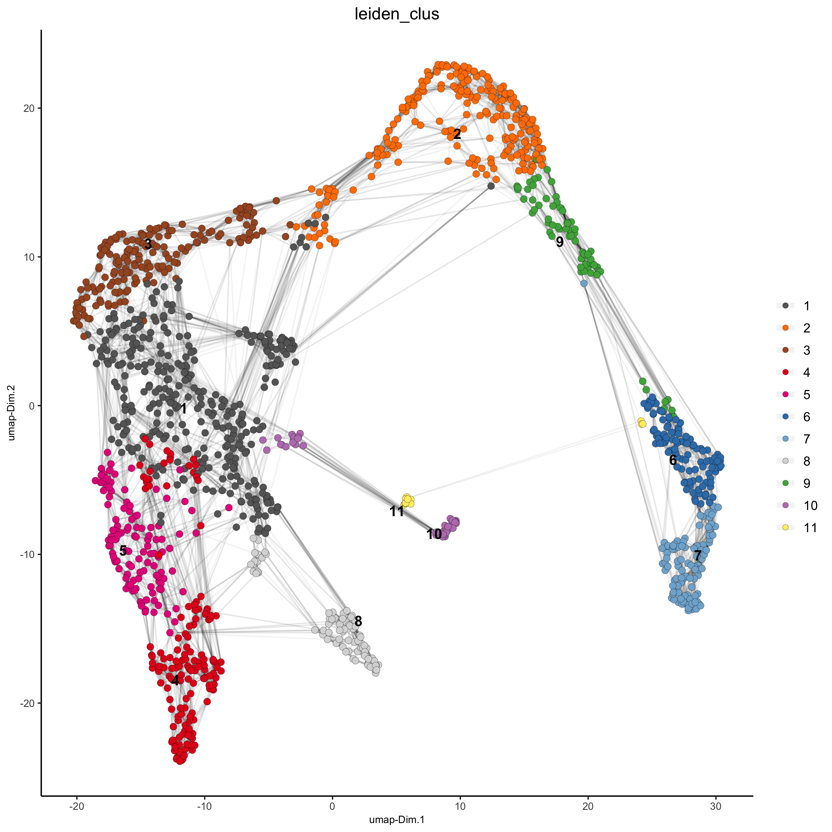
visium_kidney <- createNearestNetwork(gobject = visium_kidney, dimensions_to_use = 1:10, k = 15)
## Leiden clustering
visium_kidney <- doLeidenCluster(gobject = visium_kidney, resolution = 0.4, n_iterations = 1000)
plotUMAP(gobject = visium_kidney, cell_color = 'leiden_clus', show_NN_network = T, point_size = 2.5)

part 5: co-visualize

# expression and spatial
spatDimPlot(gobject = visium_kidney, cell_color = 'leiden_clus',
            dim_point_size = 2, spat_point_size = 2.5)

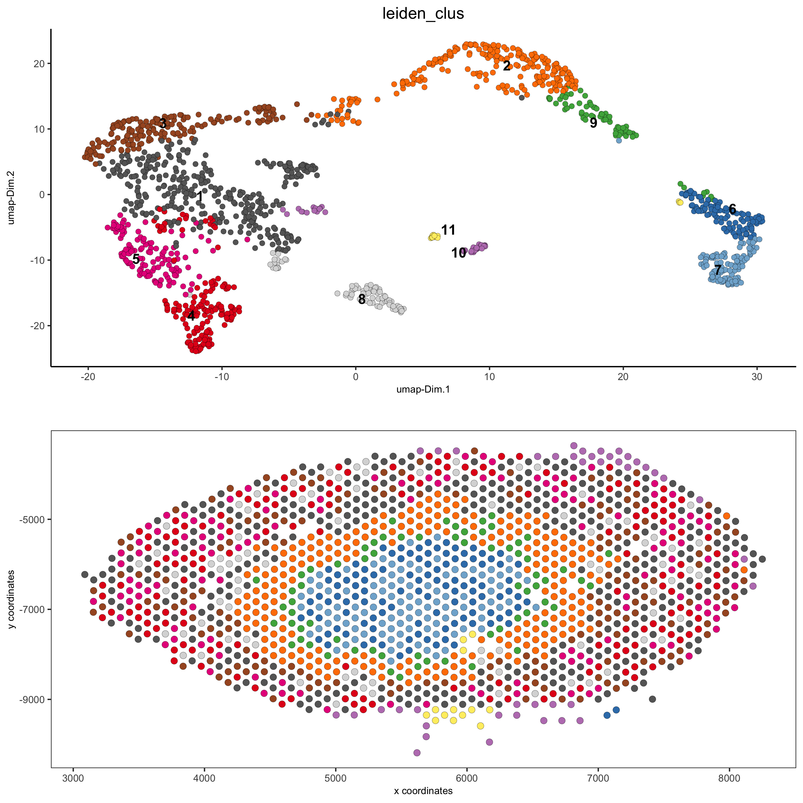
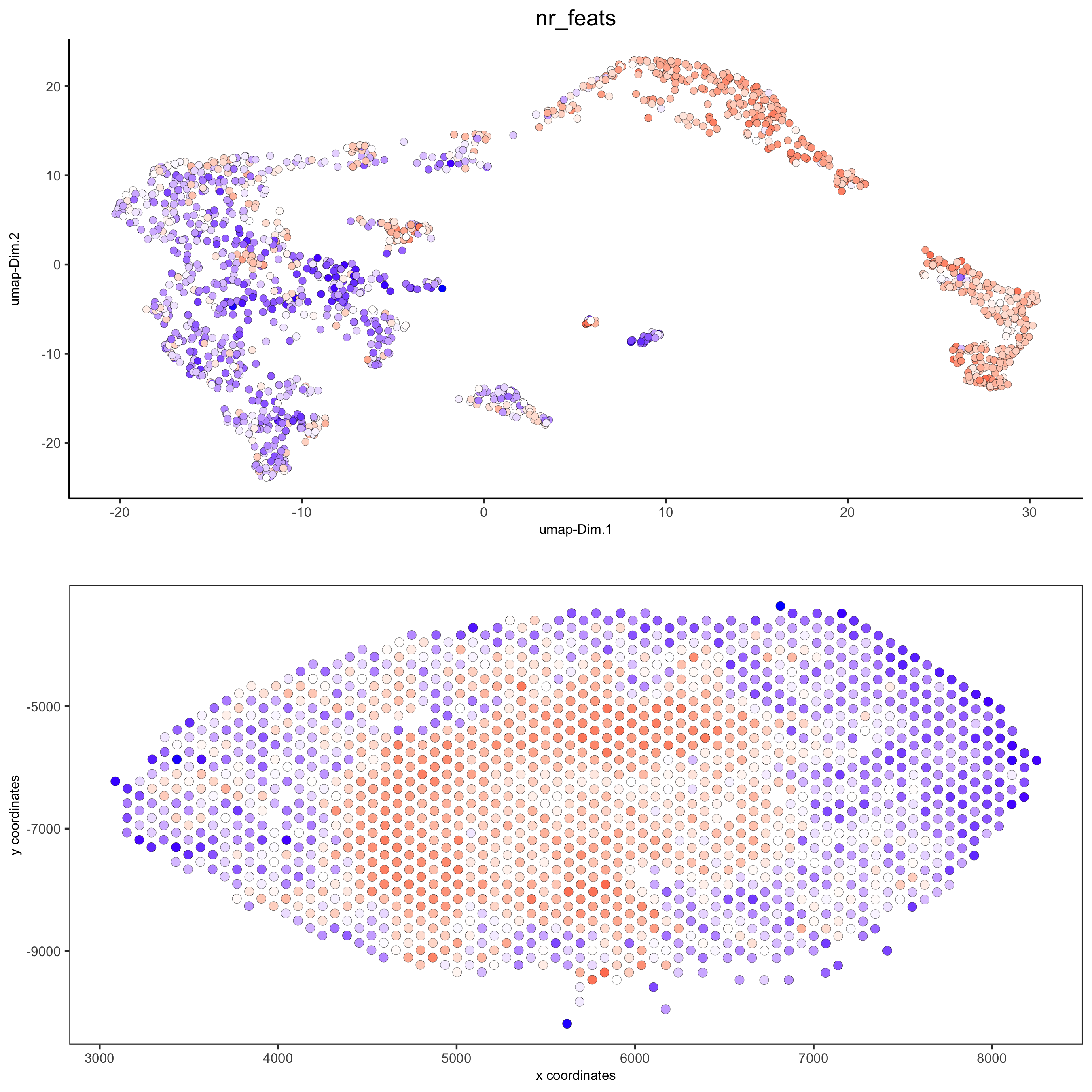
spatDimPlot(gobject = visium_kidney, cell_color = 'nr_feats', color_as_factor = F,
            dim_point_size = 2, spat_point_size = 2.5)

part 6: cell type marker gene detection

gini

gini_markers_subclusters = findMarkers_one_vs_all(gobject = visium_kidney,
                                                  method = 'gini',
                                                  expression_values = 'normalized',
                                                  cluster_column = 'leiden_clus',
                                                  min_featss = 20,
                                                  min_expr_gini_score = 0.5,
                                                  min_det_gini_score = 0.5)
topgenes_gini = gini_markers_subclusters[, head(.SD, 2), by = 'cluster']$feats

# violinplot
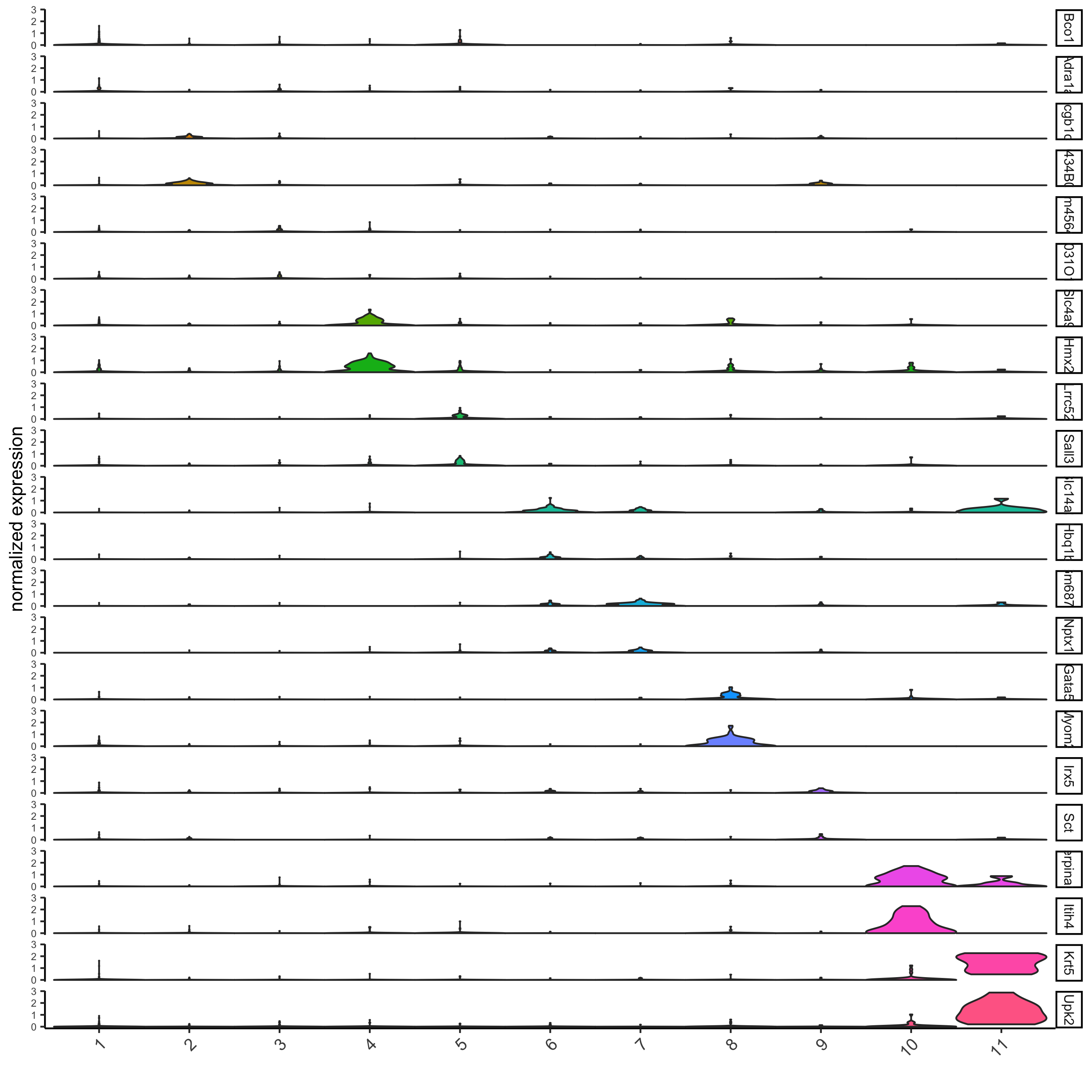
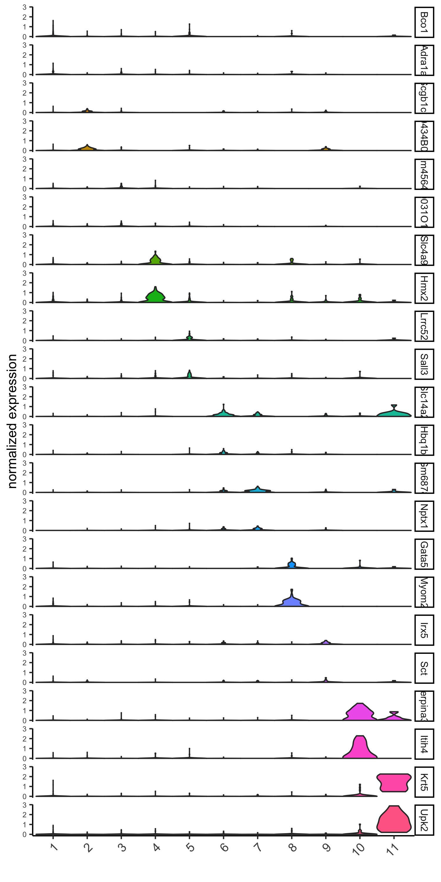
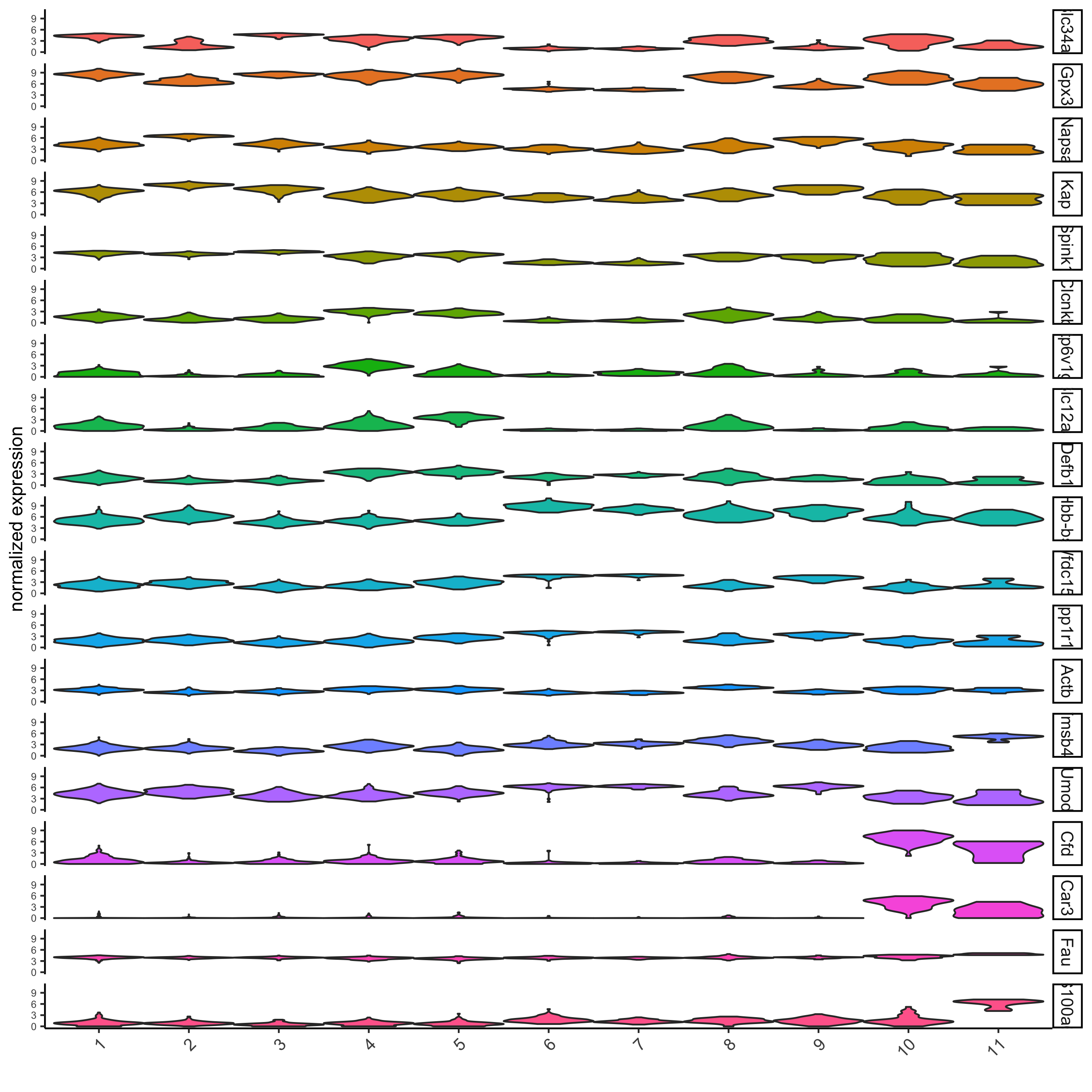
violinPlot(visium_kidney, feats = unique(topgenes_gini), cluster_column = 'leiden_clus',
           strip_text = 8, strip_position = 'right')

violinPlot(visium_kidney, feats = unique(topgenes_gini), cluster_column = 'leiden_clus',
           strip_text = 8, strip_position = 'right',
           save_param = c(save_name = '11-z1-violinplot_gini', base_width = 5, base_height = 10))

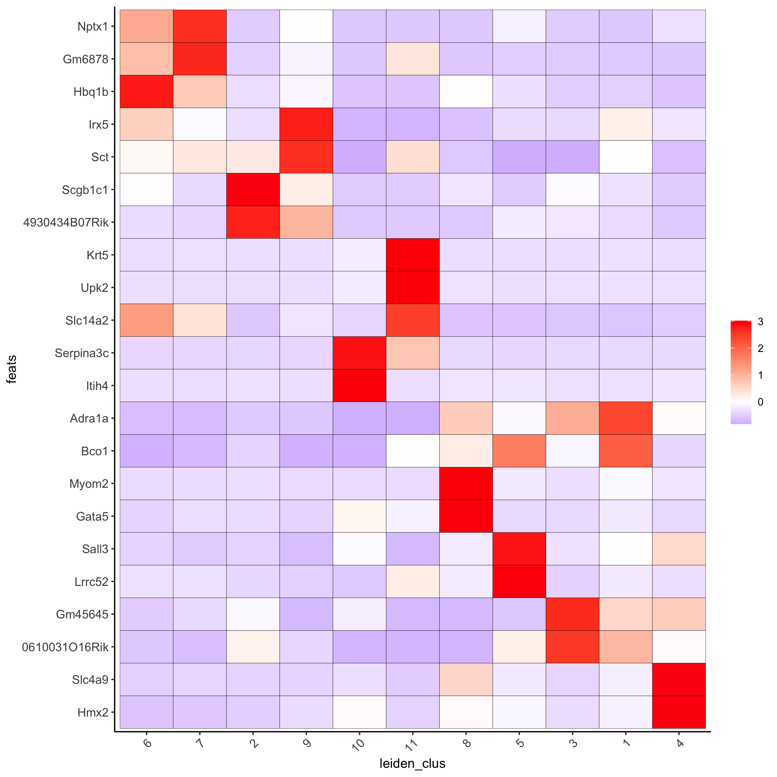
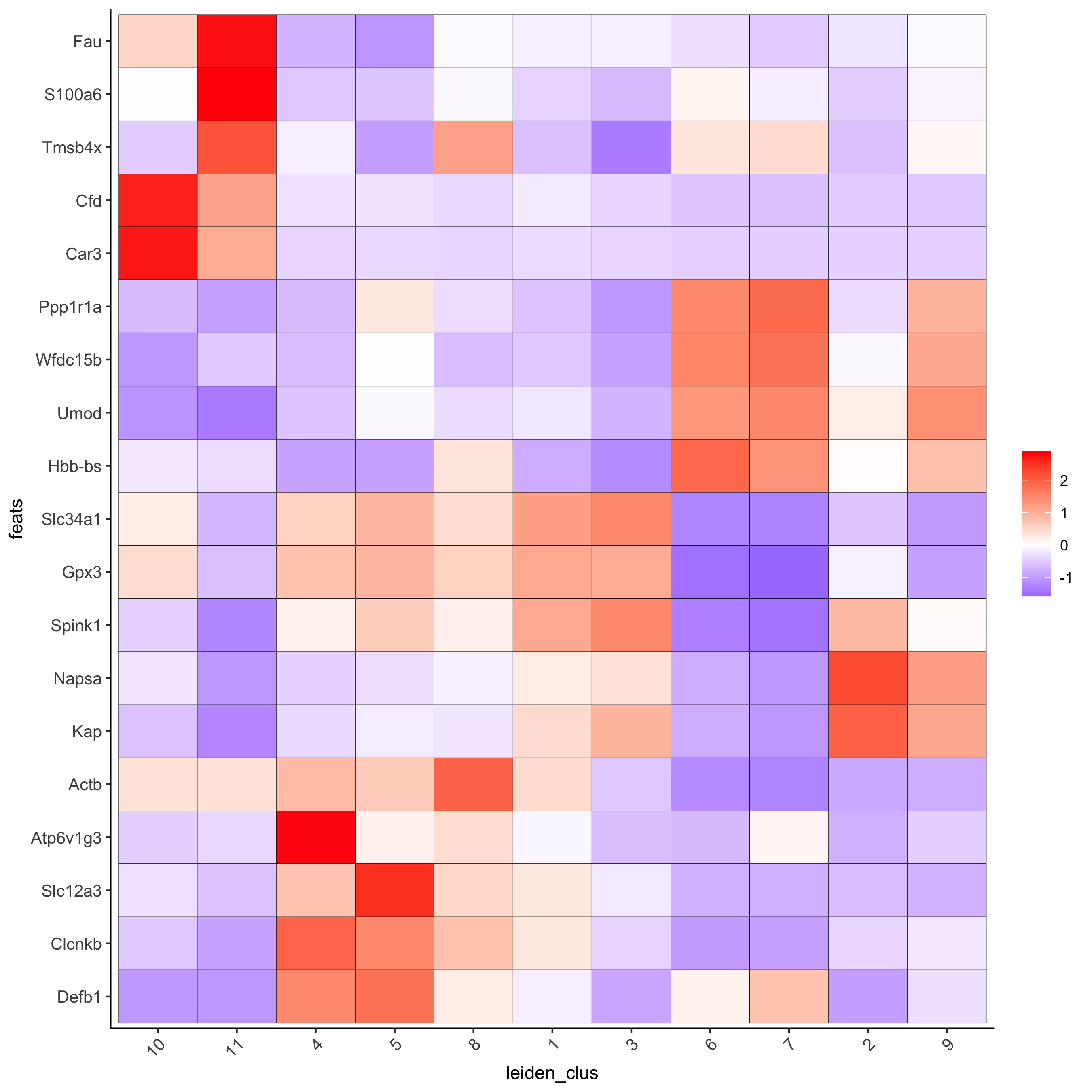
# cluster heatmap
plotMetaDataHeatmap(visium_kidney,
                    selected_feats = topgenes_gini,
                    metadata_cols = c('leiden_clus'),
                    x_text_size = 10, y_text_size = 10)

# umap plots
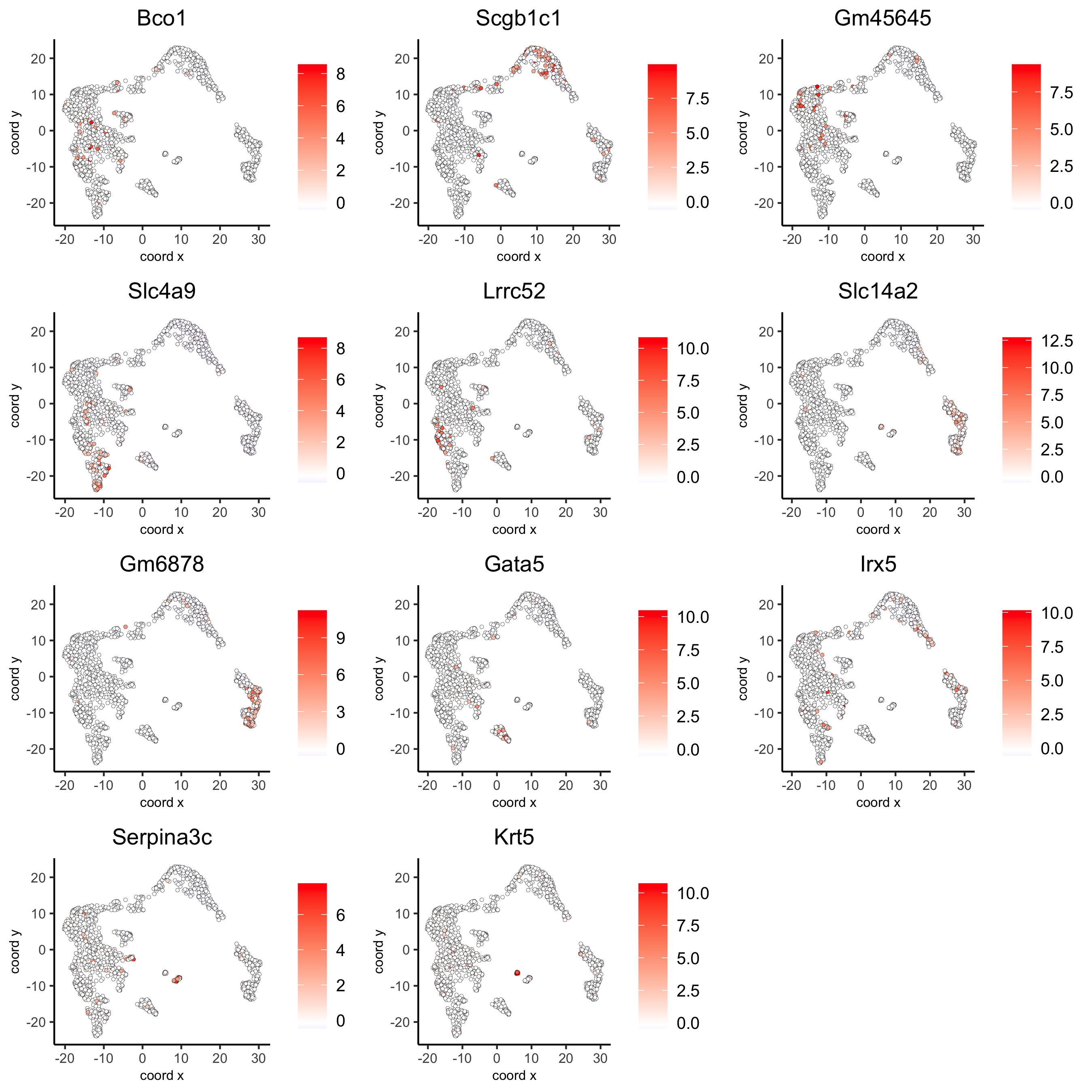
dimFeatPlot2D(visium_kidney,
              expression_values = 'scaled',
              feats = gini_markers_subclusters[, head(.SD, 1), by = 'cluster']$feats,
              cow_n_col = 3, point_size = 1)

scran

scran_markers_subclusters = findMarkers_one_vs_all(gobject = visium_kidney,
                                                   method = 'scran',
                                                   expression_values = 'normalized',
                                                   cluster_column = 'leiden_clus')
topgenes_scran = scran_markers_subclusters[, head(.SD, 2), by = 'cluster']$feats

violinPlot(visium_kidney, feats = unique(topgenes_scran),
           cluster_column = 'leiden_clus',
           strip_text = 10, strip_position = 'right')

# cluster heatmap
plotMetaDataHeatmap(visium_kidney, selected_feats = topgenes_scran,
                    metadata_cols = c('leiden_clus'))

# umap plots
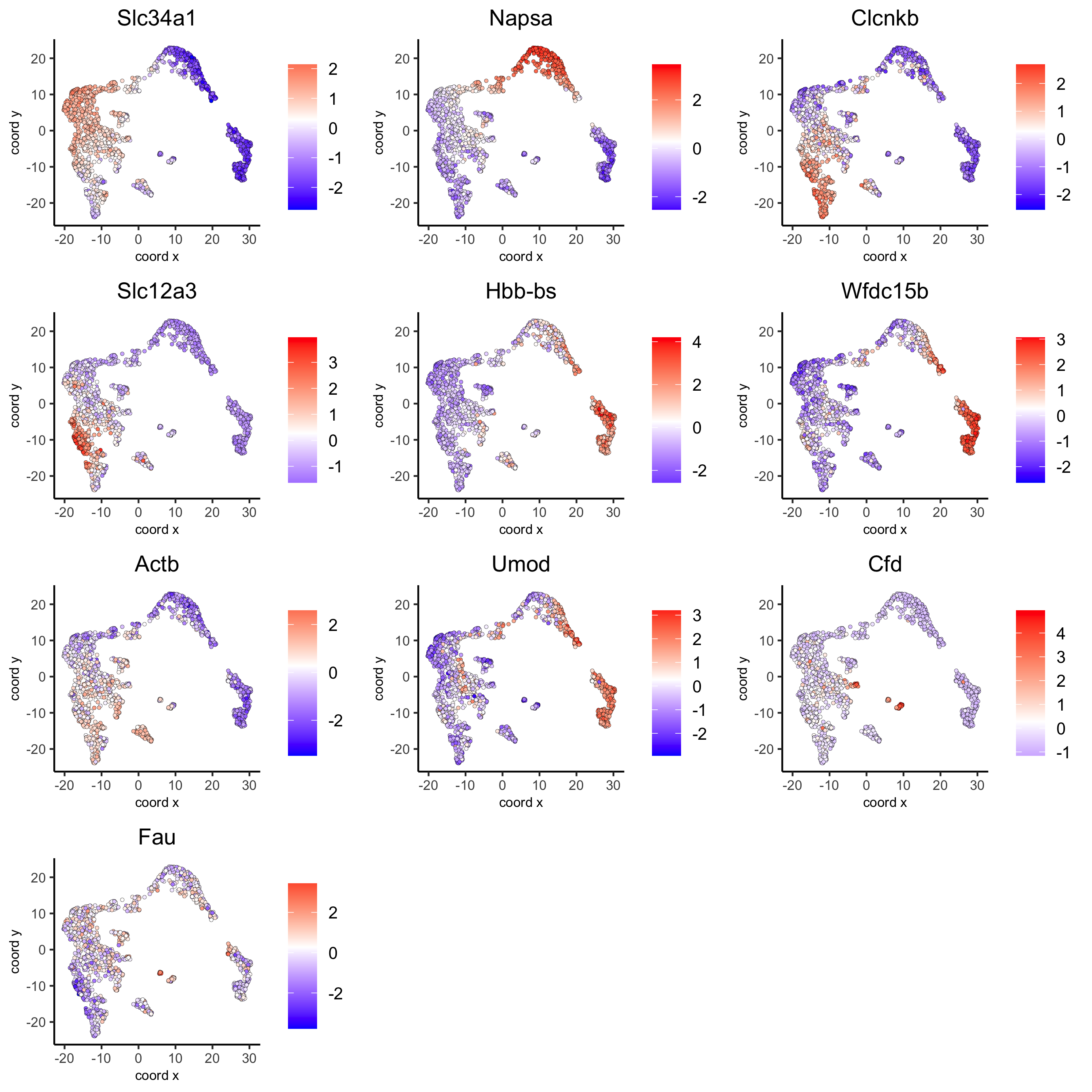
dimFeatPlot2D(visium_kidney, expression_values = 'scaled',
              feats = scran_markers_subclusters[, head(.SD, 1), by = 'cluster']$feats,
              cow_n_col = 3, point_size = 1)

part 7: cell-type annotation

Visium spatial transcriptomics does not provide single-cell resolution, making cell type annotation a harder problem. Giotto provides 3 ways to calculate enrichment of specific cell-type signature gene list:

- PAGE

- rank

- hypergeometric test

TO DO: See the mouse Visium brain dataset for an example.

part 8: spatial grid

visium_kidney <- createSpatialGrid(gobject = visium_kidney,
                                   sdimx_stepsize = 400,
                                   sdimy_stepsize = 400,
                                   minimum_padding = 0)
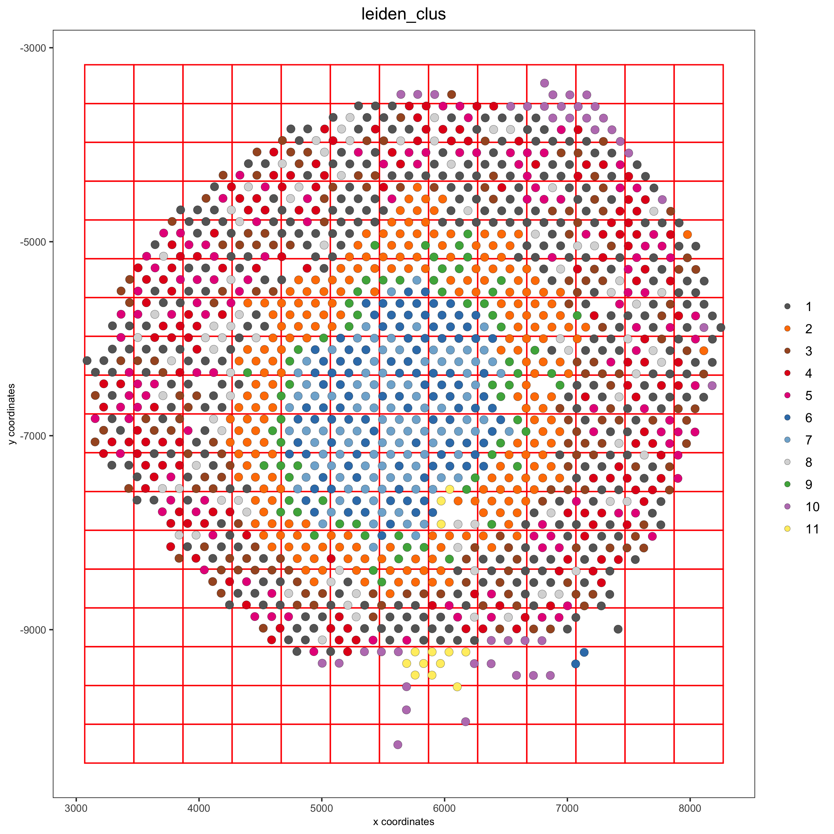
spatPlot(visium_kidney, cell_color = 'leiden_clus', show_grid = T,
         grid_color = 'red', spatial_grid_name = 'spatial_grid')

part 9: spatial network

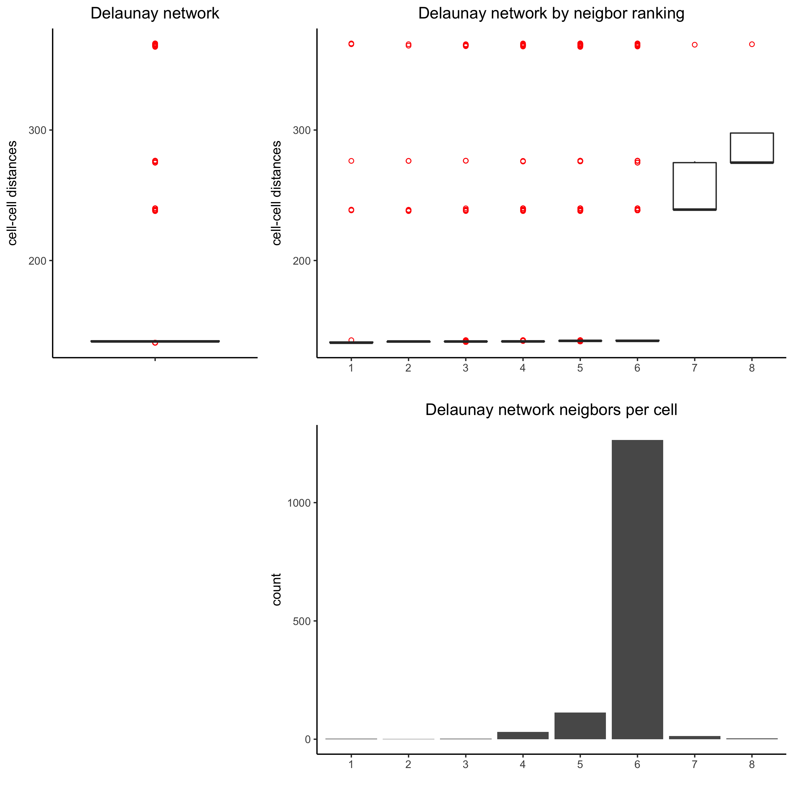
## delaunay network: stats + creation
plotStatDelaunayNetwork(gobject = visium_kidney, maximum_distance = 400)

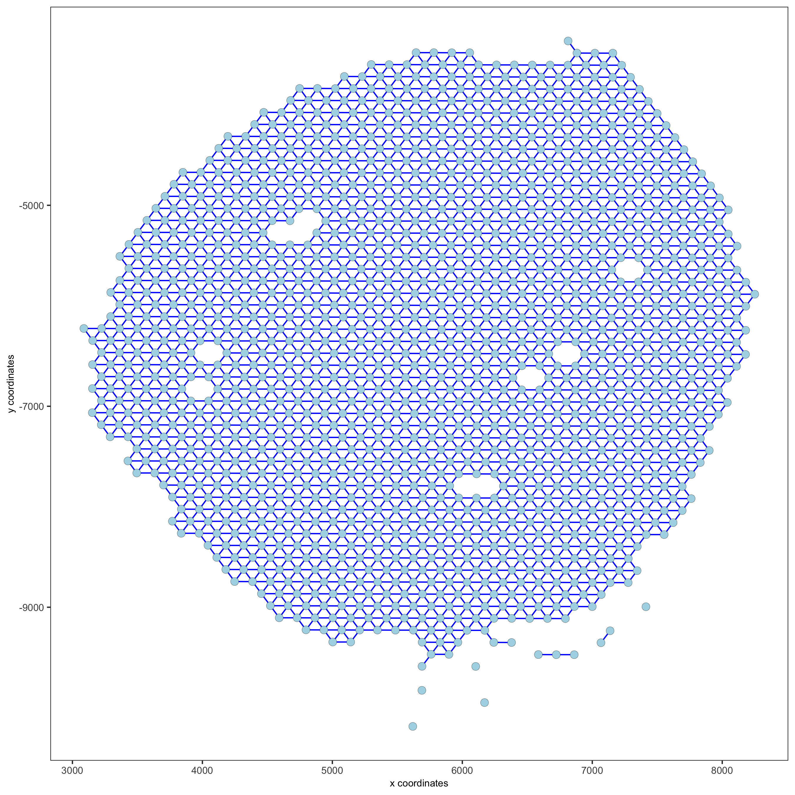
visium_kidney = createSpatialNetwork(gobject = visium_kidney, minimum_k = 0)
showNetworks(visium_kidney)
spatPlot(gobject = visium_kidney, show_network = T,
         network_color = 'blue', spatial_network_name = 'Delaunay_network')

part 10: spatial genes

Spatial genes

## kmeans binarization
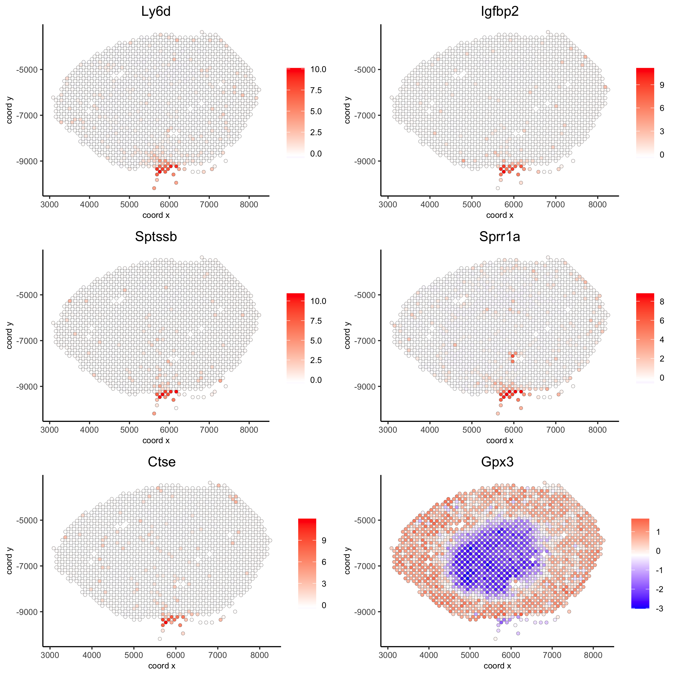
kmtest = binSpect(visium_kidney)
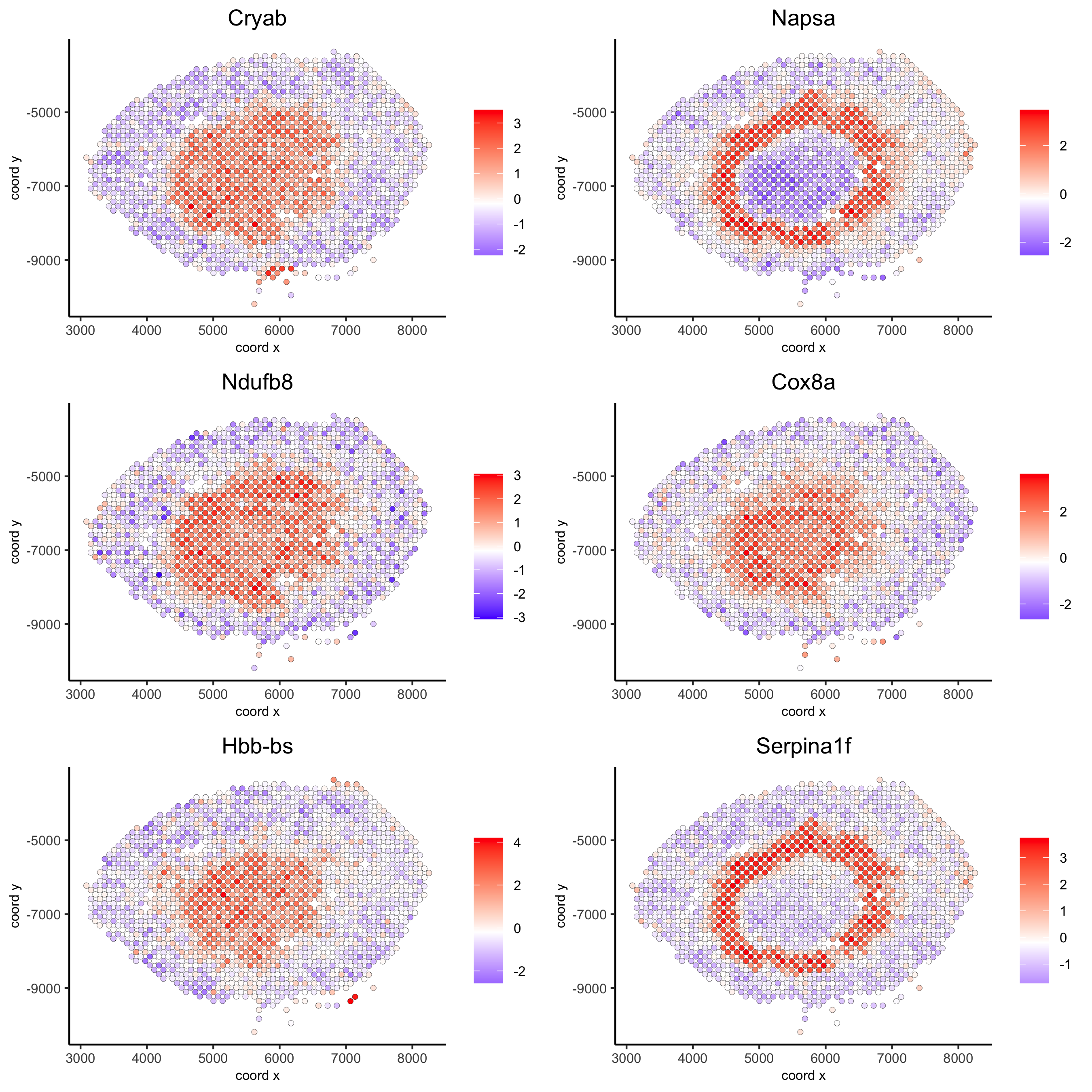
spatFeatPlot2D(visium_kidney, expression_values = 'scaled',
             feats = kmtest$feats[1:6], cow_n_col = 2, point_size = 1.5)

## rank binarization
ranktest = binSpect(visium_kidney, bin_method = 'rank')
spatFeatPlot2D(visium_kidney, expression_values = 'scaled',
             feats = ranktest$feats[1:6], cow_n_col = 2, point_size = 1.5)

Spatial co-expression patterns

## spatially correlated genes ##
ext_spatial_genes = kmtest[1:500]$feats

# 1. calculate gene spatial correlation and single-cell correlation
# create spatial correlation object
spat_cor_netw_DT = detectSpatialCorFeats(visium_kidney,
                                         method = 'network',
                                         spatial_network_name = 'Delaunay_network',
                                         subset_feats = ext_spatial_genes)

# 2. identify most similar spatially correlated genes for one gene
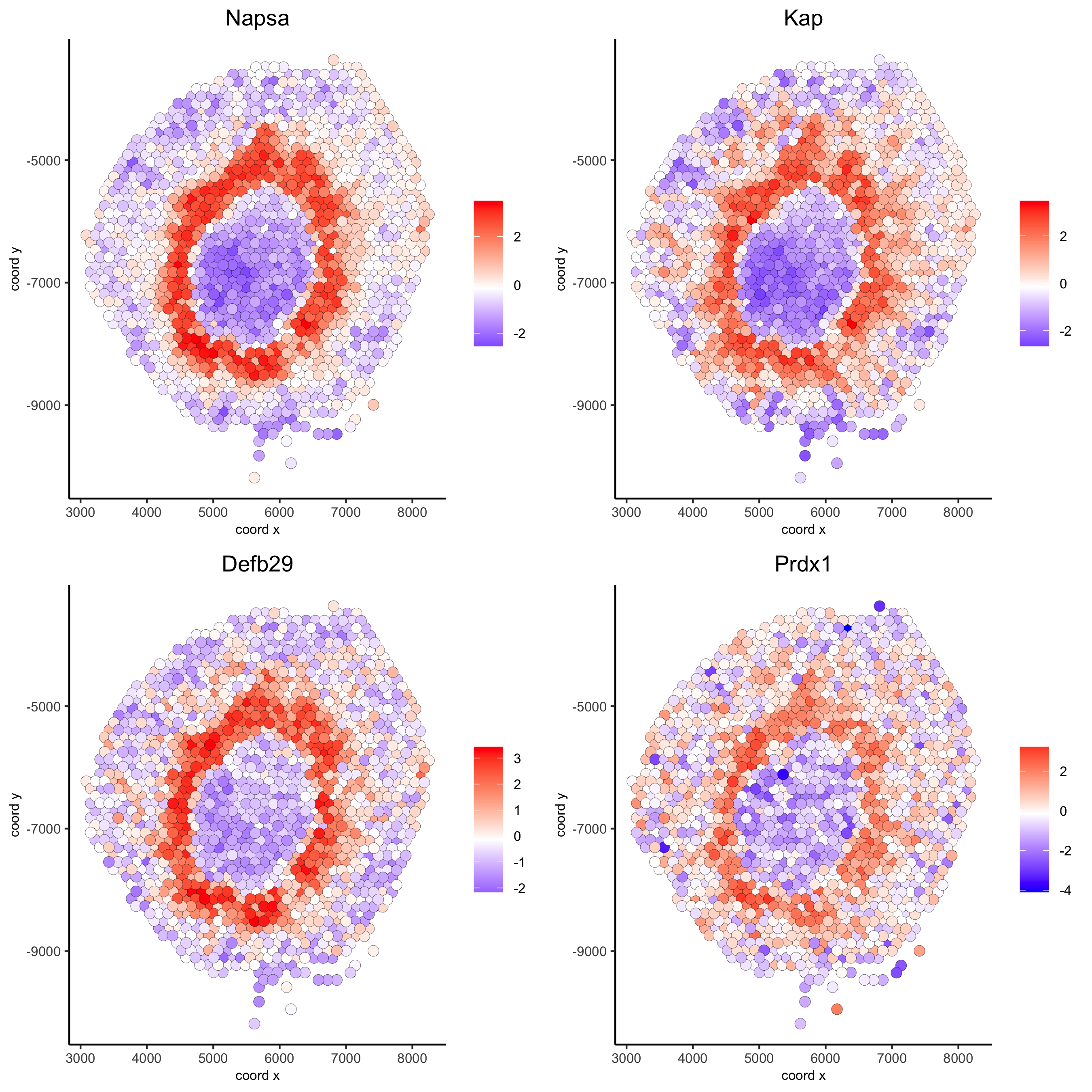
Napsa_top10_genes = showSpatialCorFeats(spat_cor_netw_DT, feats = 'Napsa', show_top_feats = 10)

spatFeatPlot2D(visium_kidney, expression_values = 'scaled',
               feats = c('Napsa', 'Kap', 'Defb29', 'Prdx1'), point_size = 3)

# 3. cluster correlated genes & visualize
spat_cor_netw_DT = clusterSpatialCorFeats(spat_cor_netw_DT, name = 'spat_netw_clus', k = 8)

heatmSpatialCorFeats(visium_kidney, spatCorObject = spat_cor_netw_DT, use_clus_name = 'spat_netw_clus',
                     save_param = c(save_name = '22-z1-heatmap_correlated_genes', save_format = 'pdf',
                                    base_height = 6, base_width = 8, units = 'cm'),
                     heatmap_legend_param = list(title = NULL))

# 4. rank spatial correlated clusters and show genes for selected clusters
netw_ranks = rankSpatialCorGroups(visium_kidney, spatCorObject = spat_cor_netw_DT, use_clus_name = 'spat_netw_clus',
                                  save_param = c(save_name = '22-z2-rank_correlated_groups',
                                                 base_height = 3, base_width = 5))

top_netw_spat_cluster = showSpatialCorFeats(spat_cor_netw_DT, use_clus_name = 'spat_netw_clus',
                                            selected_clusters = 6, show_top_feats = 1)

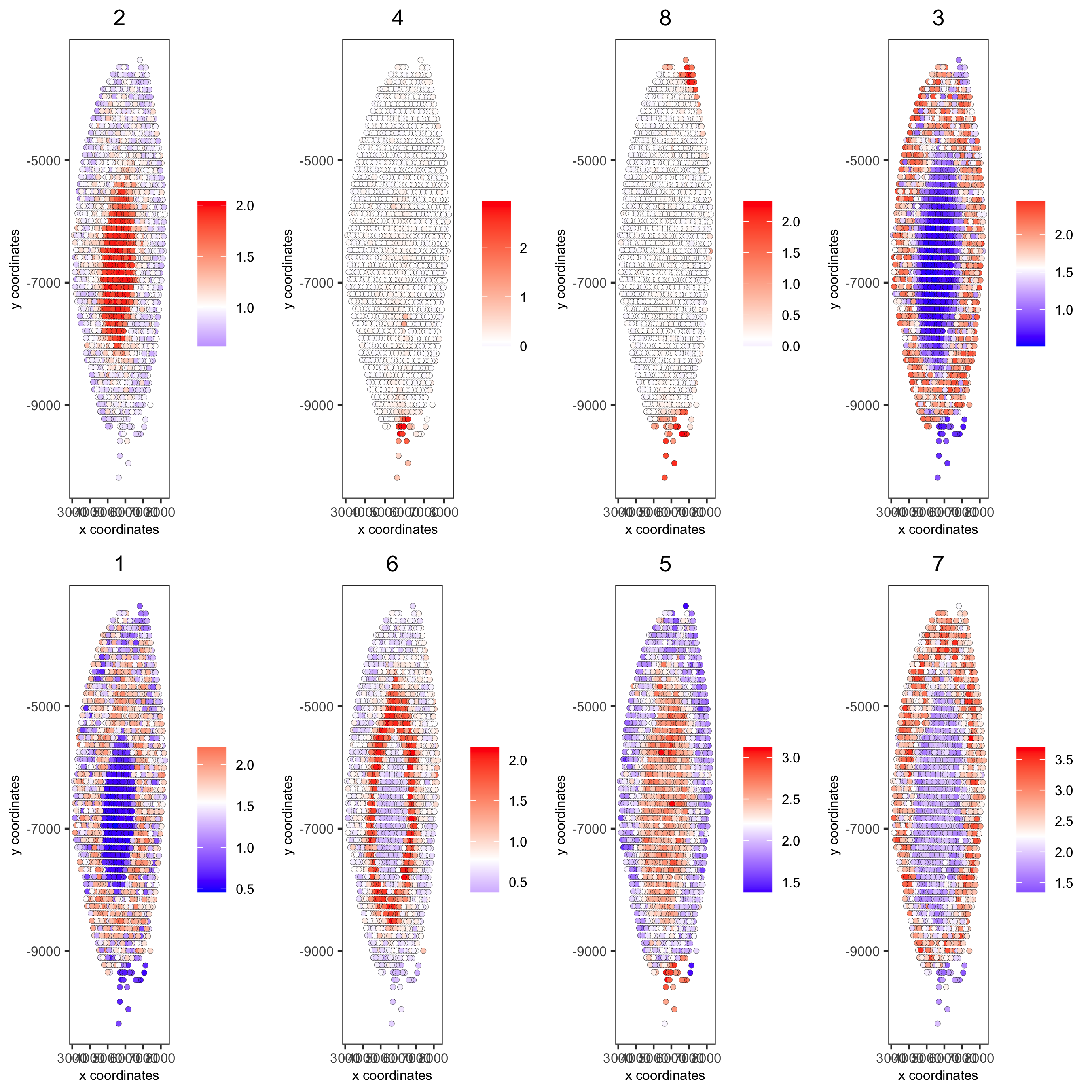
# 5. create metagene enrichment score for clusters
cluster_genes_DT = showSpatialCorFeats(spat_cor_netw_DT, use_clus_name = 'spat_netw_clus', show_top_feats = 1)
cluster_genes = cluster_genes_DT$clus; names(cluster_genes) = cluster_genes_DT$feat_ID

visium_kidney = createMetafeats(visium_kidney, feat_clusters = cluster_genes, name = 'cluster_metagene')

showGiottoSpatEnrichments(visium_kidney)

spatCellPlot(visium_kidney,
             spat_enr_names = 'cluster_metagene',
             cell_annotation_values = netw_ranks$clusters,
             point_size = 1.5, cow_n_col = 4)

part 11: HMRF domains

# HMRF requires a fully connected network!
visium_kidney = createSpatialNetwork(gobject = visium_kidney, minimum_k = 2, name = 'Delaunay_full')

# spatial genes
my_spatial_genes <- kmtest[1:100]$feats

# do HMRF with different betas
hmrf_folder = paste0(results_folder,'/','HMRF_results/')
if(!file.exists(hmrf_folder)) dir.create(hmrf_folder, recursive = T)

# if Rscript is not found, you might have to create a symbolic link, e.g.
# cd /usr/local/bin
# sudo ln -s /Library/Frameworks/R.framework/Resources/Rscript Rscript
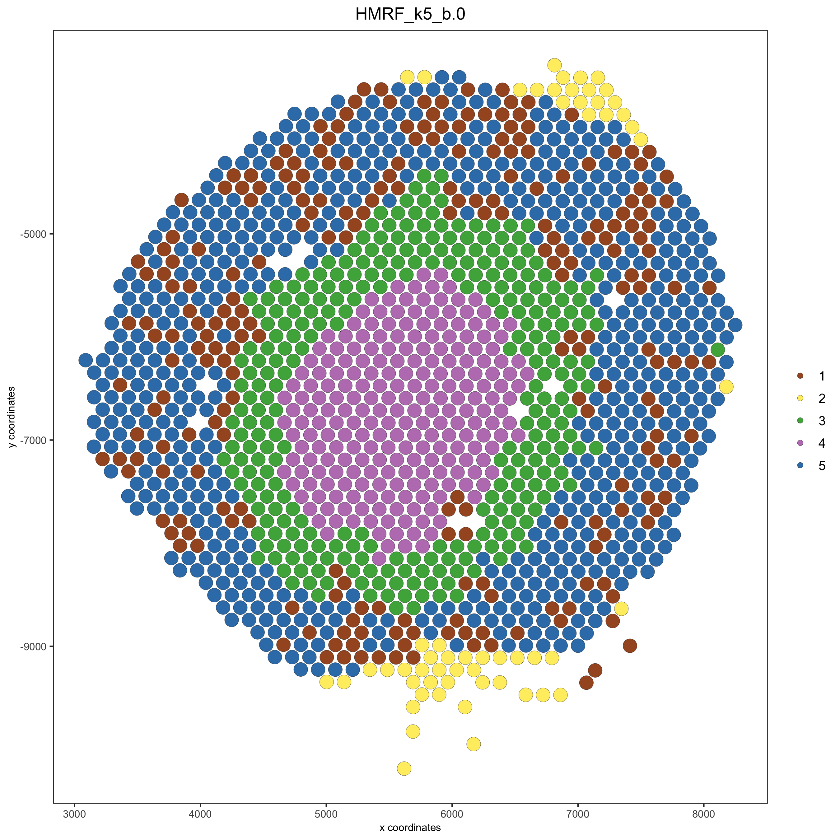
HMRF_spatial_genes = doHMRF(gobject = visium_kidney,
                            expression_values = 'scaled',
                            spatial_network_name = 'Delaunay_full',
                            spatial_genes = my_spatial_genes,
                            k = 5,
                            betas = c(0, 1, 6),
                            output_folder = paste0(hmrf_folder, '/', 'Spatial_genes/SG_topgenes_k5_scaled'))

## alternative way to view HMRF results
#results = writeHMRFresults(gobject = ST_test,
#                           HMRFoutput = HMRF_spatial_genes,
#                           k = 5, betas_to_view = seq(0, 25, by = 5))
#ST_test = addCellMetadata(ST_test, new_metadata = results, by_column = T, column_cell_ID = 'cell_ID')


## add HMRF of interest to giotto object
visium_kidney = addHMRF(gobject = visium_kidney,
                        HMRFoutput = HMRF_spatial_genes,
                        k = 5, betas_to_add = c(0, 2),
                        hmrf_name = 'HMRF')

## visualize
spatPlot(gobject = visium_kidney, cell_color = 'HMRF_k5_b.0', point_size = 5)

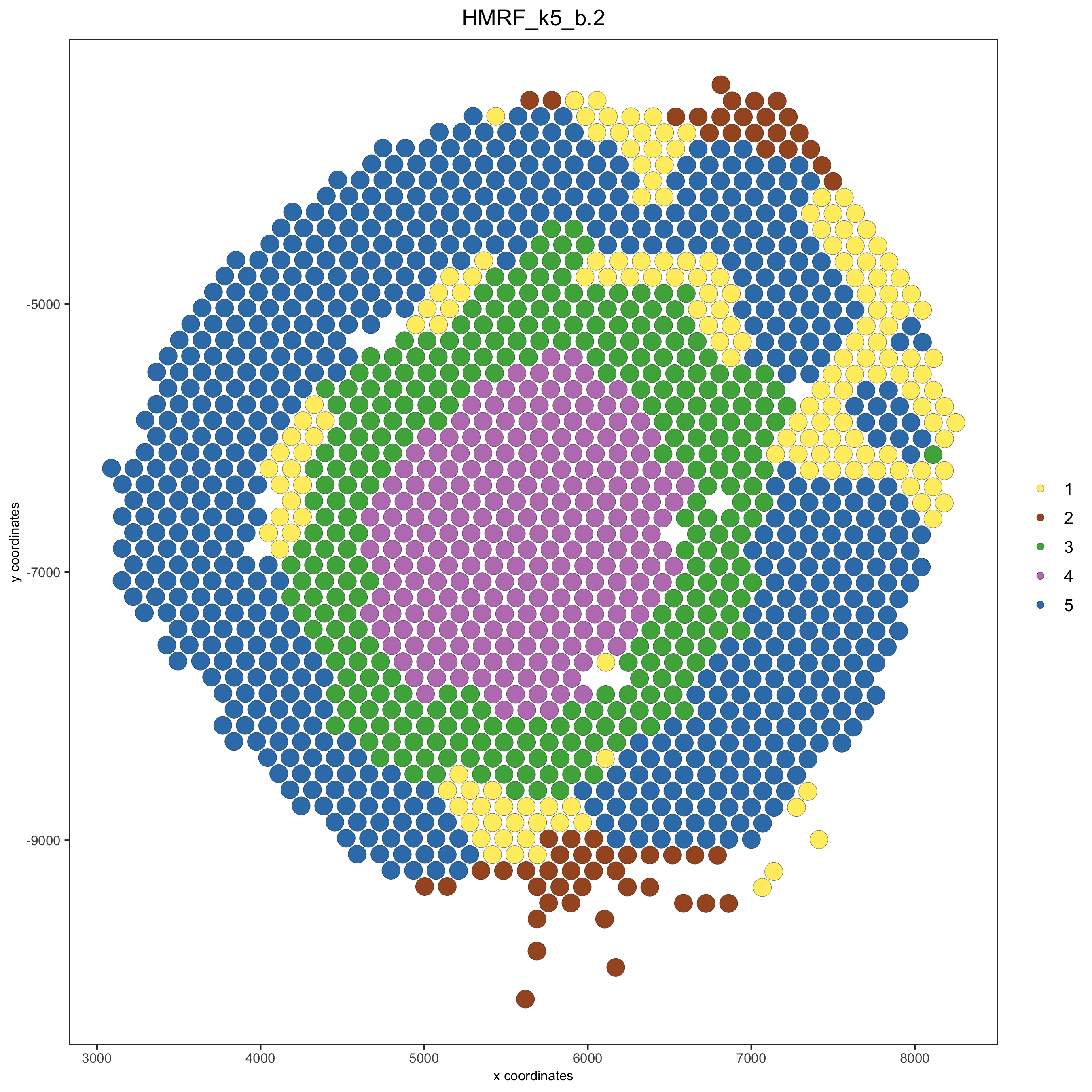
spatPlot(gobject = visium_kidney, cell_color = 'HMRF_k5_b.2', point_size = 5)

Export and create Giotto Viewer

# check which annotations are available
combineMetadata(visium_kidney)

# select annotations, reductions and expression values to view in Giotto Viewer
viewer_folder = paste0(results_folder, '/', 'mouse_visium_kidney_viewer')

exportGiottoViewer(gobject = visium_kidney,
                   output_directory = viewer_folder,
                   factor_annotations = c('in_tissue',
                                          'leiden_clus'),
                   numeric_annotations = c('nr_feats'),
                   dim_reductions = c('tsne', 'umap'),
                   dim_reduction_names = c('tsne', 'umap'),
                   expression_values = 'scaled',
                   expression_rounding = 2,
                   overwrite_dir = T)