Clustering#
- Date:
4/12/23
1 Dataset explanation#
This tutorial walks through the dimension reduction and clustering capabilities of Giotto and begins with the Giotto Object processed in the previous tutorial, data processing. For convenience, the code to create this object is provided below. However, new users are encouraged to review the data processing tutorial prior to beginning this tutorial.
This tutorial uses a SeqFISH+ dataset of a murine cortex and subventrical zone. A complete walkthrough of that dataset can be found here. To download the data used to create the Giotto Object below, please ensure that wget is installed locally.
2 Start Giotto#
# Ensure Giotto Suite is installed
if(!"Giotto" %in% installed.packages()) {
  devtools::install_github("drieslab/Giotto@suite")
}
library(Giotto)

# Ensure Giotto Data is installed
if(!"GiottoData" %in% installed.packages()) {
  devtools::install_github("drieslab/GiottoData")
}
library(GiottoData)

# Ensure the Python environment for Giotto has been installed
genv_exists = checkGiottoEnvironment()
if(!genv_exists){
  # The following command need only be run once to install the Giotto environment
  installGiottoEnvironment()
}
3 Creating and Processing a Giotto Object#
# Specify path from which data may be retrieved/stored
data_directory = paste0(getwd(),'/gobject_clustering_data/')
# alternatively, "/path/to/where/the/data/lives/"

# Specify path to which results may be saved
results_directory = paste0(getwd(),'/gobject_clustering_results/')
# alternatively, "/path/to/store/the/results/"

# Optional: Specify a path to a Python executable within a conda or miniconda
# environment. If set to NULL (default), the Python executable within the previously
# installed Giotto environment will be used.
my_python_path = NULL # alternatively, "/local/python/path/python" if desired.

getSpatialDataset(dataset = 'seqfish_SS_cortex', directory = data_directory, method = 'wget')
# Set Giotto instructions
instrs = createGiottoInstructions(save_plot = TRUE,
                                  show_plot = TRUE,
                                  save_dir = results_directory,
                                  python_path = my_python_path)
# Create giotto object from provided paths
expr_path = paste0(data_directory, "cortex_svz_expression.txt")
loc_path = paste0(data_directory, "cortex_svz_centroids_coord.txt")
meta_path = paste0(data_directory, "cortex_svz_centroids_annot.txt")


# This dataset contains multiple field of views which need to be stitched together.

# First, merge location and additional metadata
SS_locations = data.table::fread(loc_path)
cortex_fields = data.table::fread(meta_path)
SS_loc_annot = data.table::merge.data.table(SS_locations, cortex_fields, by = 'ID')
SS_loc_annot[, ID := factor(ID, levels = paste0('cell_',1:913))]
data.table::setorder(SS_loc_annot, ID)

# Create a file with offset information
my_offset_file = data.table::data.table(field = c(0, 1, 2, 3, 4, 5, 6),
                                        x_offset = c(0, 1654.97, 1750.75, 1674.35, 675.5, 2048, 675),
                                        y_offset = c(0, 0, 0, 0, -1438.02, -1438.02, 0))

# Create a file to stitch the multiple fields of view together
stitch_file = stitchFieldCoordinates(location_file = SS_loc_annot,
                                     offset_file = my_offset_file,
                                     cumulate_offset_x = T,
                                     cumulate_offset_y = F,
                                     field_col = 'FOV',
                                     reverse_final_x = F,
                                     reverse_final_y = T)
stitch_file    = stitch_file[,.(ID, X_final, Y_final)]
stitch_file$ID = as.character(stitch_file$ID) # ID must be a character vector
my_offset_file = my_offset_file[,.(field, x_offset_final, y_offset_final)]

# Create Giotto object
testobj <- createGiottoObject(expression = expr_path,
                              spatial_locs = stitch_file,
                              offset_file = my_offset_file,
                              instructions = instrs)
# Add additional annotation if wanted
testobj = addCellMetadata(testobj,
                          new_metadata = cortex_fields,
                          by_column = T,
                          column_cell_ID = 'ID')

# Subset data to the cortex field of views in a new Giotto object
cell_metadata = getCellMetadata(testobj)[]
cortex_cell_ids = cell_metadata[FOV %in% 0:4]$cell_ID
testobj = subsetGiotto(testobj, cell_ids = cortex_cell_ids)
# Process the Giotto object, filtering, normalization, adding statistics and correcting for covariates
testobj <- processGiotto(testobj,
                        filter_params = list(expression_threshold = 1,
                                             feat_det_in_min_cells = 100,
                                             min_det_feats_per_cell = 10),
                        norm_params = list(norm_methods = 'standard',
                                           scale_feats = TRUE,
                                           scalefactor = 6000),
                        stat_params = list(expression_values = 'normalized'),
                        adjust_params = list(expression_values = c('normalized'),
                                             covariate_columns = 'nr_feats'))
4 Dimension Reduction and PCA#
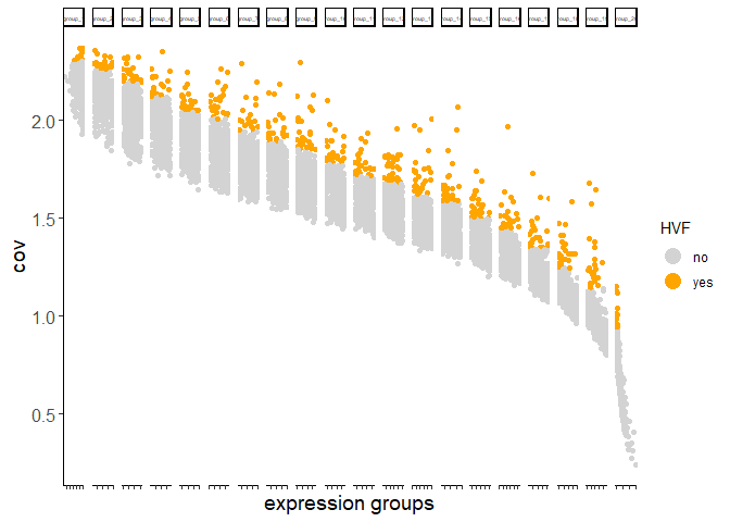
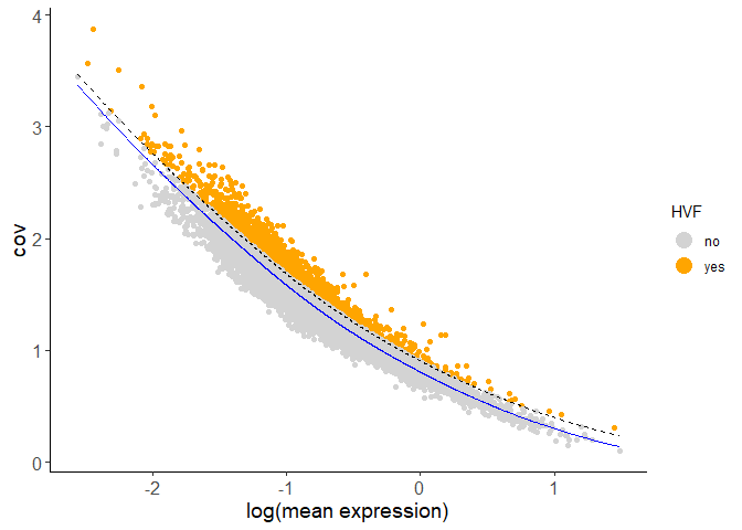
Highly variable features (genes) may be computed based on high coefficient of variance within groups, variance of pearson residuals for each gene, or loess regression predictions. Specify the desired computation with the method parameter.
Calculate HVF using coefficient of variance within groups:
testobj <- calculateHVF(gobject = testobj, method = 'cov_groups')
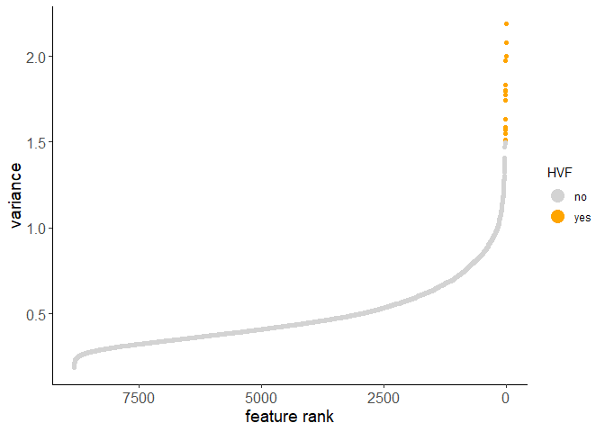
Calculate HVF using variance of Pearson residuals:
testobj <- calculateHVF(gobject = testobj, method = 'var_p_resid')
Calculate HVF using the loess regression prediction model:
testobj <- calculateHVF(gobject = testobj, method = 'cov_loess')
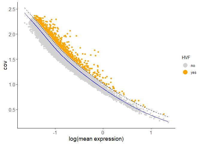
PCA can be run based on the highly variable genes. After PCA, a tSNE, a UMAP, or both may be run. For this example, highly variable genes have been identified using Loess Regression predictions.
## Select genes highly variable genes that fit specified statistics
# These are both found within feature metadata
feature_metadata = getFeatureMetadata(testobj)[]
featgenes = feature_metadata[hvf == 'yes' & perc_cells > 4 & mean_expr_det > 0.5]$feat_ID

## run PCA on expression values (default)
testobj <- runPCA(gobject = testobj, feats_to_use = featgenes, scale_unit = F, center = F)
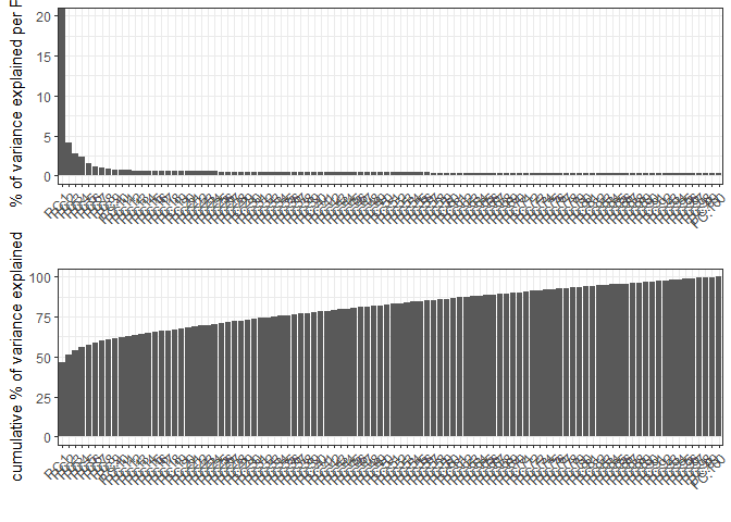
# plot a scree plot
screePlot(testobj)
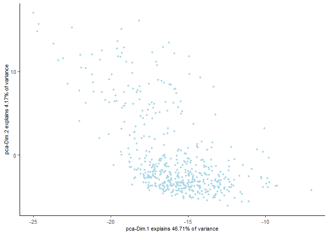
# Plot a PCA
plotPCA(gobject = testobj)
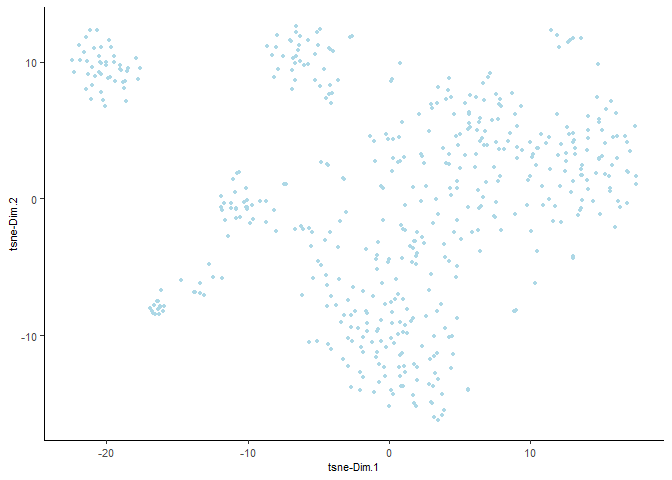
Run a tSNE based on PCA dimension reduction and view it in a plot
testobj <- runtSNE(testobj, dimensions_to_use = 1:15)
plotTSNE(gobject = testobj)
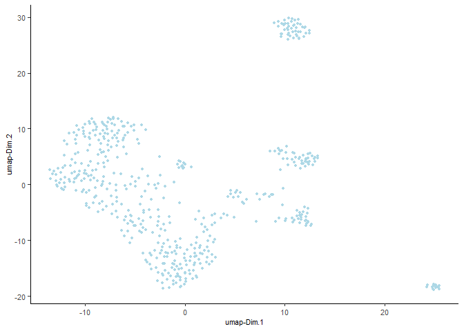
Run a UMAP based on PCA dimension reduction and view pre-clustering UMAP
testobj <- runUMAP(testobj, dimensions_to_use = 1:15)
plotUMAP(gobject = testobj)
5 Clustering#
Cells may be clustered into distinct groups based on feature expression. To cluster, the Giotto Object must contain data that has undergone PCA dimension reduction, either tSNE or UMAP dimension reduction, and have a neighbor network.
Create a shared nearest neighbor network (sNN), where k is the number of k neighbors to use:
testobj <- createNearestNetwork(gobject = testobj, type = "sNN", dimensions_to_use = 1:15, k = 15)
Note the argument ‘type’ is specified for emphasis here. It takes ‘sNN’ as its default argument; Giotto also supports k nearest neighbor clustering (kNN). Simply specify ‘type = “kNN”’ to create a kNN instead of a sNN.
Cells can be clustered in Giotto using k-means, Leiden, or Louvain clustering. These clustering algorithms return cluster information within cell_metadata, which is named accordingly by default. The name may be changed by providing the name argument, as shown in the code chunk below.
Naming clusters allows for clusters of various resolutions to be created if desired, and assists in visualization; cluster names may be provided as an argument to cell_color within plotUMAP for enhanced visualization.
## k-means clustering
testobj <- doKmeans(gobject = testobj, dim_reduction_to_use = 'pca')
## Leiden clustering - increase the resolution to increase the number of clusters
testobj <- doLeidenCluster(gobject = testobj,
resolution = 0.4,
n_iterations = 1000,
name = 'leiden_0.4_1000')
## Louvain clustering - increase the resolution to increase the number of clusters
# The version argument may be changed to 'multinet' to run a Louvain algorithm
# from the multinet package in R.
testobj <- doLouvainCluster(gobject = testobj,
version = 'community',
resolution = 0.4)
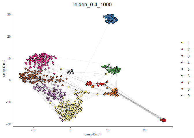
#Plot UMAP post-clustering to visualize Leiden clusters
plotUMAP(gobject = testobj,
cell_color = 'leiden_0.4_1000',
show_NN_network = T,
point_size = 2.5)
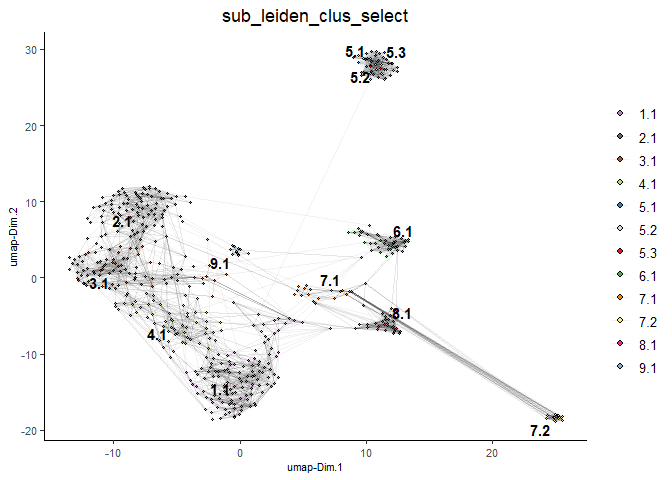
Clusters of interest can be further sub-clustered. Choose the clusters to be sub-clustered with the selected_clusters argument. Note that the same HVF method selection and PCA parameters are used here for consistent sub-clustering.
## Leiden subclustering for specified clusters
testobj = doLeidenSubCluster(gobject = testobj,
                             cluster_column = 'leiden_0.4_1000',
                             resolution = 0.2,
                             k_neighbors = 10,
                             hvf_param = list(method = 'cov_loess',
                                              difference_in_cov = 0.1),
                             pca_param = list(expression_values = 'normalized',
                                              scale_unit = F,
                                              center = F),
                             nn_param = list(dimensions_to_use = 1:5),
                             selected_clusters = c(5, 6, 7),
                             name = 'sub_leiden_clus_select')
#Plot a UMAP to visualize sub-clusters
plotUMAP(gobject = testobj, cell_color = 'sub_leiden_clus_select', show_NN_network = T)
6 Session Info#
sessionInfo()
R version 4.2.2 (2022-10-31 ucrt)
Platform: x86_64-w64-mingw32/x64 (64-bit)
Running under: Windows 10 x64 (build 22621)

Matrix products: default

locale:
[1] LC_COLLATE=English_United States.utf8
[2] LC_CTYPE=English_United States.utf8
[3] LC_MONETARY=English_United States.utf8
[4] LC_NUMERIC=C
[5] LC_TIME=English_United States.utf8

attached base packages:
[1] stats     graphics  grDevices utils     datasets  methods   base

other attached packages:
[1] GiottoData_0.1.0 Giotto_3.2.1

loaded via a namespace (and not attached):
 [1] ggrepel_0.9.2         rsvd_1.0.5            Rcpp_1.0.10
 [4] here_1.0.1            lattice_0.20-45       FNN_1.1.3.2
 [7] png_0.1-7             rprojroot_2.0.3       digest_0.6.30
[10] utf8_1.2.3            R6_2.5.1              stats4_4.2.2
[13] evaluate_0.20         ggplot2_3.4.1         pillar_1.9.0
[16] rlang_1.1.0           rstudioapi_0.14       data.table_1.14.6
[19] irlba_2.3.5.1         S4Vectors_0.36.2      Matrix_1.5-1
[22] reticulate_1.26       rmarkdown_2.21        textshaping_0.3.6
[25] labeling_0.4.2        BiocParallel_1.32.6   Rtsne_0.16
[28] igraph_1.4.1          uwot_0.1.14           munsell_0.5.0
[31] beachmat_2.14.0       DelayedArray_0.24.0   compiler_4.2.2
[34] BiocSingular_1.14.0   xfun_0.38             pkgconfig_2.0.3
[37] systemfonts_1.0.4     BiocGenerics_0.44.0   htmltools_0.5.4
[40] tidyselect_1.2.0      tibble_3.2.1          IRanges_2.32.0
[43] codetools_0.2-18      matrixStats_0.63.0    fansi_1.0.4
[46] dplyr_1.1.1           withr_2.5.0           rappdirs_0.3.3
[49] grid_4.2.2            jsonlite_1.8.3        gtable_0.3.3
[52] lifecycle_1.0.3       magrittr_2.0.3        scales_1.2.1
[55] ScaledMatrix_1.6.0    cli_3.4.1             dbscan_1.1-11
[58] farver_2.1.1          limma_3.54.2          ragg_1.2.4
[61] generics_0.1.3        vctrs_0.6.1           cowplot_1.1.1
[64] RColorBrewer_1.1-3    tools_4.2.2           glue_1.6.2
[67] MatrixGenerics_1.10.0 parallel_4.2.2        fastmap_1.1.0
[70] yaml_2.3.7            colorspace_2.1-0      terra_1.7-18
[73] knitr_1.42