Saving Giotto Plots#
- Date:
last-modified 04/14/23
1 Saving Spatial Data in Plots#
Please see the Configuration and Giotto Object vignettes before walking through this tutorial.
R/Rstudio and Giotto provide different ways to save spatial data. Here, a giottoObject will be created without using giottoInstructions so that the save parameters for plotting functions within Giotto as well as the default saving methods built into R/Rstudio may be emphasized here. Note that for plotting functions, all parameters available to the save_param argument may be found by running showSaveParameters().
# Ensure Giotto Suite is installed.
if(!"Giotto" %in% installed.packages()) {
  devtools::install_github("drieslab/Giotto@suite")
}

# Ensure GiottoData, a small, helper module for tutorials, is installed.
if(!"GiottoData" %in% installed.packages()) {
  devtools::install_github("drieslab/GiottoData")
}
library(Giotto)
# Ensure the Python environment for Giotto has been installed.
genv_exists = checkGiottoEnvironment()
if(!genv_exists){
  # The following command need only be run once to install the Giotto environment.
  installGiottoEnvironment()
}
2 Creating the Giotto Object without Instructions:#
Since the focus of this vignette is saving methods, the giottoObject will not be created with giottoInstructions. See Giotto Object for further intuition on working with a giottoObject that has been provided instructions.
library(Giotto)
library(GiottoData)

data_directory = paste0(getwd(),'/')

# Download dataset
getSpatialDataset(dataset = 'osmfish_SS_cortex', directory = data_directory, method = 'wget')

# Specify path to files
osm_exprs = paste0(data_directory, "osmFISH_prep_expression.txt")
osm_locs = paste0(data_directory, "osmFISH_prep_cell_coordinates.txt")
meta_path = paste0(data_directory, "osmFISH_prep_cell_metadata.txt")

## CREATE GIOTTO OBJECT with expression data and location data
my_gobject <- createGiottoObject(expression = osm_exprs,
                                 spatial_locs = osm_locs)

metadata = data.table::fread(file = meta_path)
my_gobject = addCellMetadata(my_gobject, new_metadata = metadata,
                             by_column = T, column_cell_ID = 'CellID')
3 Examples#
3.1 Standard R save methods#
Note that by default, plotting functions will return a plot object that may be saved or further manipulated.
### Manually save plot as a PDF in the current working directory:
save_path = paste0(getwd(),'/first_plot.pdf')
# This function serves only to ensure the following lines run consecutively.
save_pdf_plot <- function(){
pdf(file = save_path, width = 7, height = 7)
pl = spatPlot(my_gobject)
dev.off()
}
save_pdf_plot()
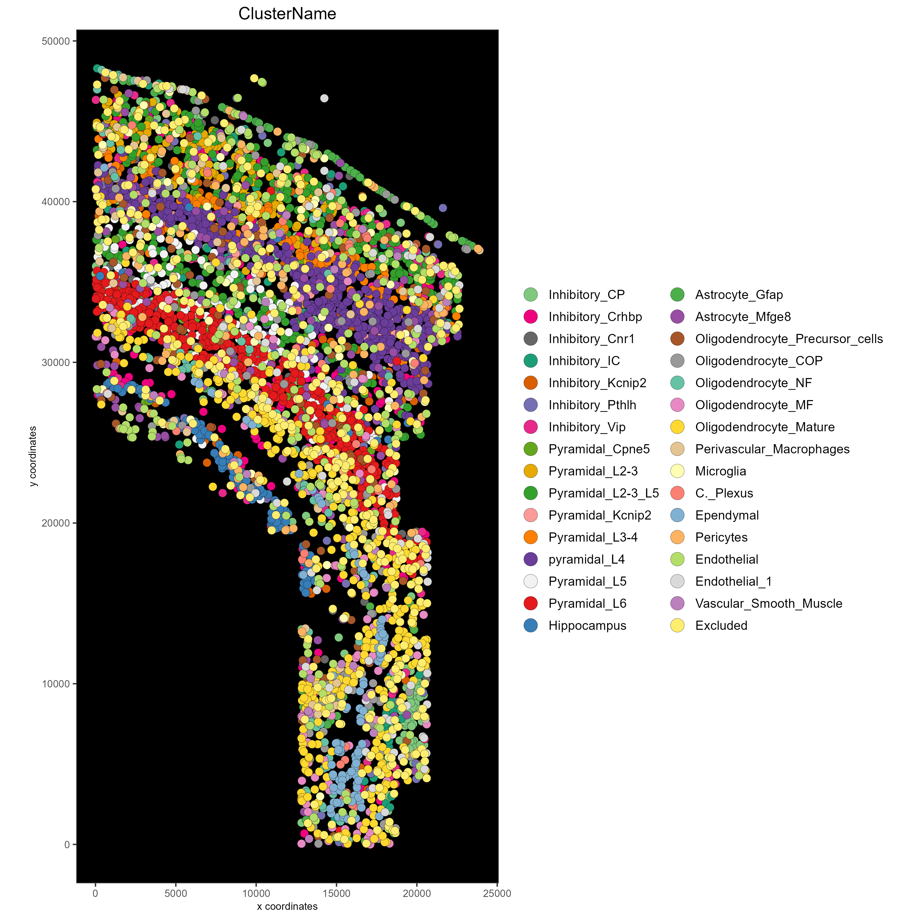
### Plot clusters, edit plot object, then save using the ggplot add-on, cowplot:
mypl = spatPlot(gobject = my_gobject,
cell_color = 'ClusterName')
# Add a black background
mypl = mypl + theme(panel.background = element_rect(fill ='black'),
panel.grid = element_blank())
# Add a legend
mypl = mypl + guides(fill = guide_legend(override.aes = list(size=5)))
# Save in the current working directory
cowplot::save_plot(plot = mypl,
filename = 'clusters_black.png',
path = getwd(),
device = png(),
dpi = 300,
base_height = 10,
base_width = 10)
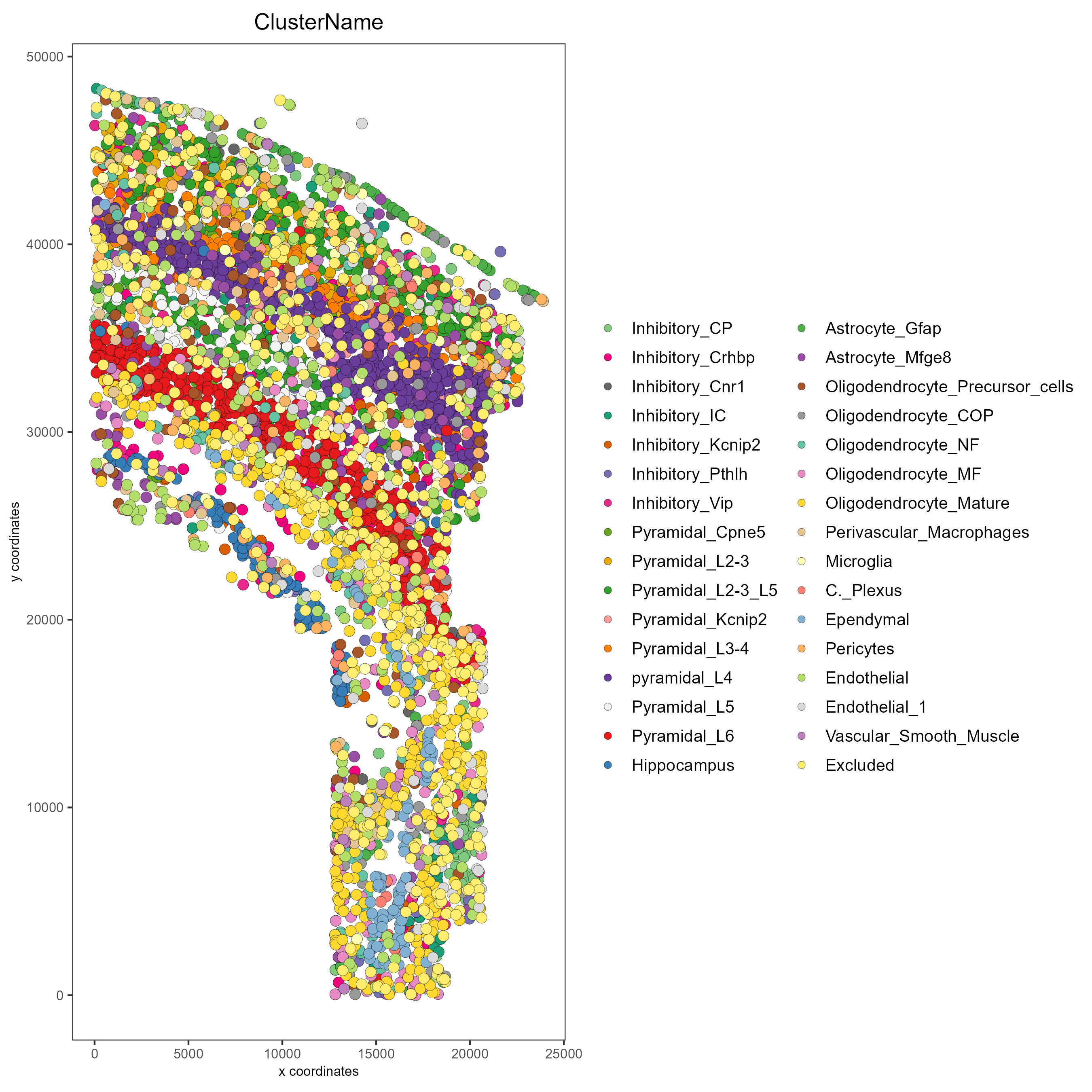
3.2 Save plot directly to the default folder#
The default save folder is the current working directory. This will be the case if instructions are not provided, or if a save_dir is not specified within giottoInstructions. See the createGiottoInstructions documentation and Giotto Object for default arguments and more details.
# Plot clusters and save to default folder
spatPlot(my_gobject,
         cell_color = 'ClusterName',
         save_plot = TRUE)
3.3 Save plot directly, but overwrite default save parameters#
In this example, assume it is desired that the plot is: - Shown in the console - Not returned as an object from the plotting function call - Saved in a subdirectory of the current working directory as a .png file with a dpi of 200, height of 9 inches, and width of 9 inches. - Saved with the file name “my_name”
# Specify new subdirectory name
results_directory =  'my_subfolder/'

# Plot clusters, create, and save to a new subdirectory with specifications above.
spatPlot(my_gobject,
         cell_color = 'ClusterName',
         save_plot = TRUE,
         return_plot = FALSE,
         save_param = list(save_folder = results_directory, # Create subdirectory
                           save_name = 'my_name',
                           save_format = 'png',
                           units = 'in',
                           base_height = 9,
                           base_width = 9))

3.4 Just view the plot#
# Plot without saving
spatPlot(my_gobject,
         cell_color = 'ClusterName',
         save_plot = FALSE, return_plot = FALSE, show_plot = T)
3.5 Just save the plot (FASTEST for large datasets!)#
# only saves the plot
spatPlot(my_gobject,
         cell_color = 'ClusterName',
         save_plot = TRUE, return_plot = FALSE, show_plot = FALSE,
         save_param = list(save_name = 'only_save'))
