mini3D STARmap#
library(Giotto)
Install Python Modules#
To run this vignette you need to install all of the necessary Python modules.
Important
Python module installation can be done either automatically via our installation tool (from within R) (see step 2.2A) or manually (see step 2.2B).
See Part 2.2 Giotto-Specific Python Packages of our Giotto Installation section for step-by-step instructions.
Optional: Set Giotto Instructions#
# to automatically save figures in save_dir set save_plot to TRUE
temp_dir = getwd()
temp_dir = '~/Temp/'
myinstructions = createGiottoInstructions(save_dir = temp_dir,
                      save_plot = TRUE,
                      show_plot = FALSE)
1. Giotto Object#
Minimum Requirements:#
Matrix with expression information (or path to)
x,y(,z) coordinates for cells or spots (or path to)
# giotto object
expr_path = system.file("extdata", "starmap_expr.txt.gz", package = 'Giotto')
loc_path = system.file("extdata", "starmap_cell_loc.txt", package = 'Giotto')
starmap_mini <- createGiottoObject(raw_exprs = expr_path,
                spatial_locs = loc_path,
                instructions = myinstructions)
How to work with Giotto instructions that are part of your Giotto object:
Show the instructions associated with your Giotto object with showGiottoInstructions
Change one or more instructions with changeGiottoInstructions
Replace all instructions at once with replaceGiottoInstructions
Read or get a specific giotto instruction with readGiottoInstructions
Note: The python path can only be set once in an R session. See the **reticulate package* for more information.*
# show instructions associated with giotto object (starmap_mini)
showGiottoInstructions(starmap_mini)
2. Processing Steps#
Filter genes and cells based on detection frequencies
Normalize expression matrix (log transformation, scaling factor and/or z-scores)
Add cell and gene statistics (optional)
Adjust expression matrix for technical covariates or batches (optional). These results will be stored in the custom slot.
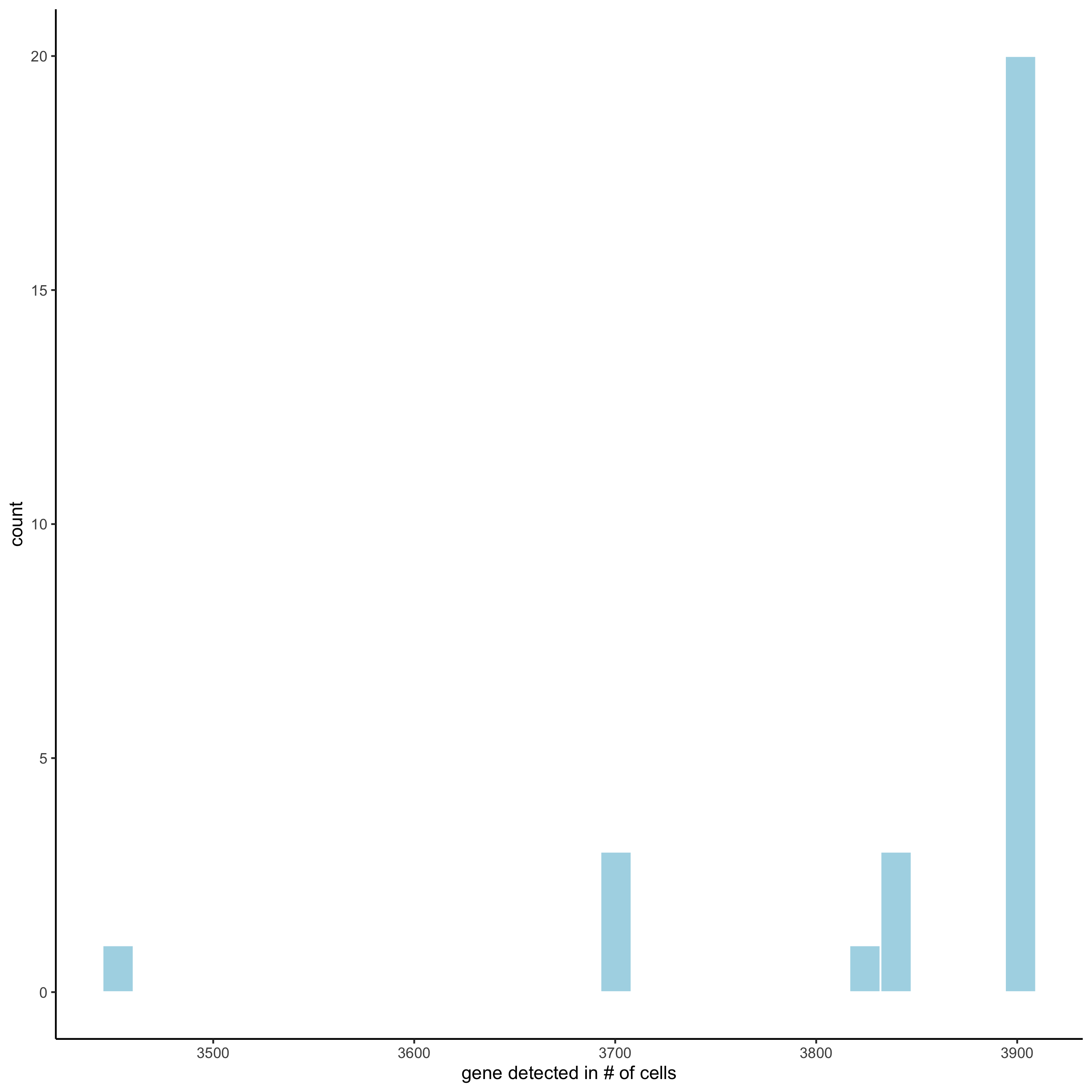
filterDistributions(starmap_mini, detection = 'genes',
        save_param = list(save_name = '2_a_filtergenes'))
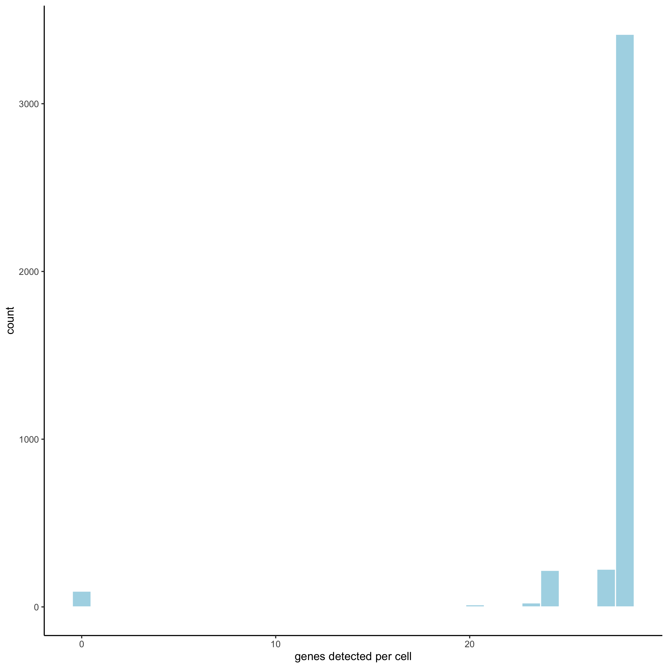
filterDistributions(starmap_mini, detection = 'cells',
        save_param = list(save_name = '2_b_filtercells'))
filterCombinations(starmap_mini,
       expression_thresholds = c(1),
       gene_det_in_min_cells = c(50, 100, 200),
       min_det_genes_per_cell = c(20, 28, 28),
       save_param = list(save_name = '2_c_filtercombos'))
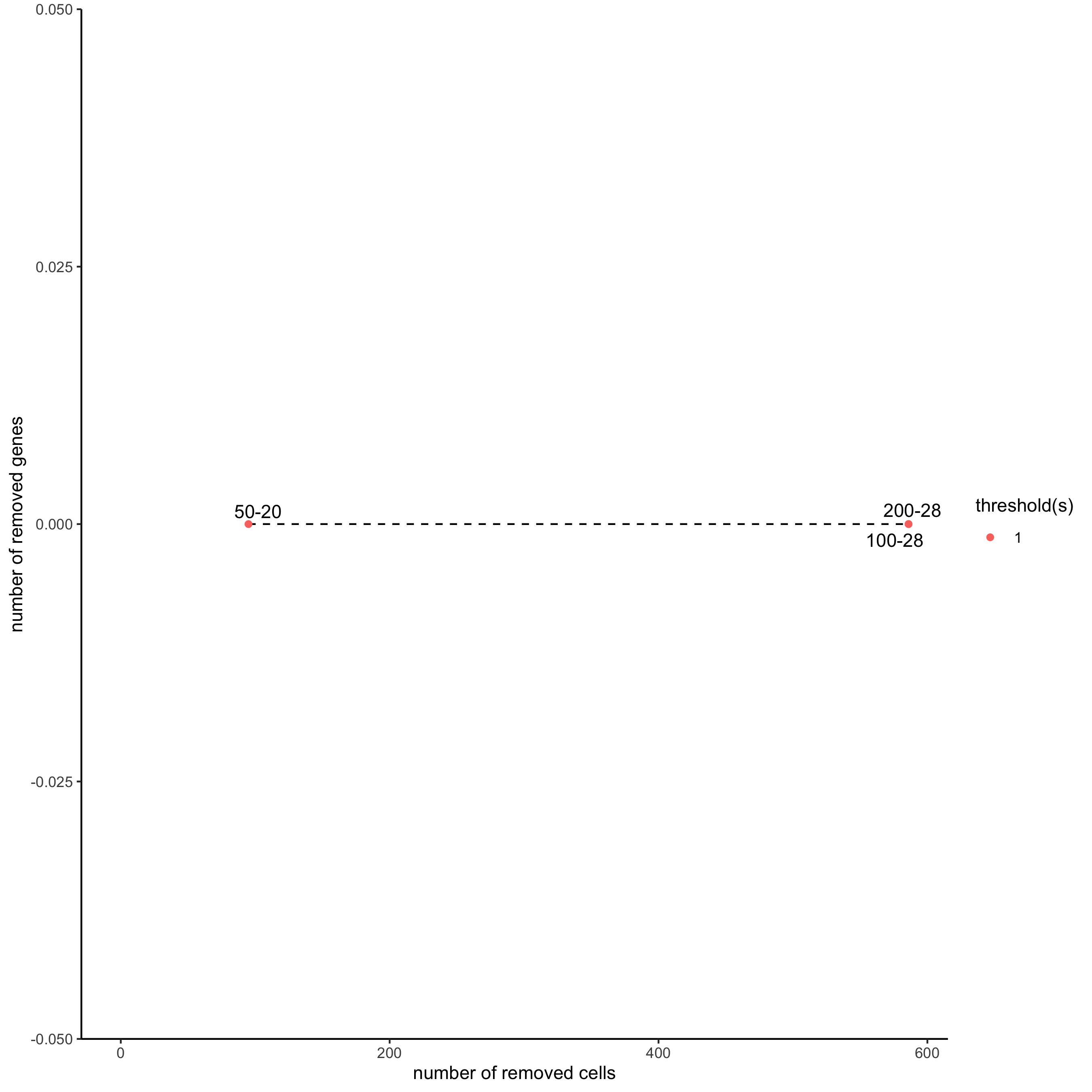
starmap_mini <- filterGiotto(gobject = starmap_mini,
           expression_threshold = 1,
           gene_det_in_min_cells = 50,
           min_det_genes_per_cell = 20,
           expression_values = c('raw'),
           verbose = T)
starmap_mini <- normalizeGiotto(gobject = starmap_mini,
            scalefactor = 6000, verbose = T)
starmap_mini <- addStatistics(gobject = starmap_mini)
3. Dimension Reduction#
Identify highly variable genes (HVG)
Perform PCA
Identify number of significant prinicipal components (PCs)
Run UMAP and/or TSNE on PCs (or directly on matrix)
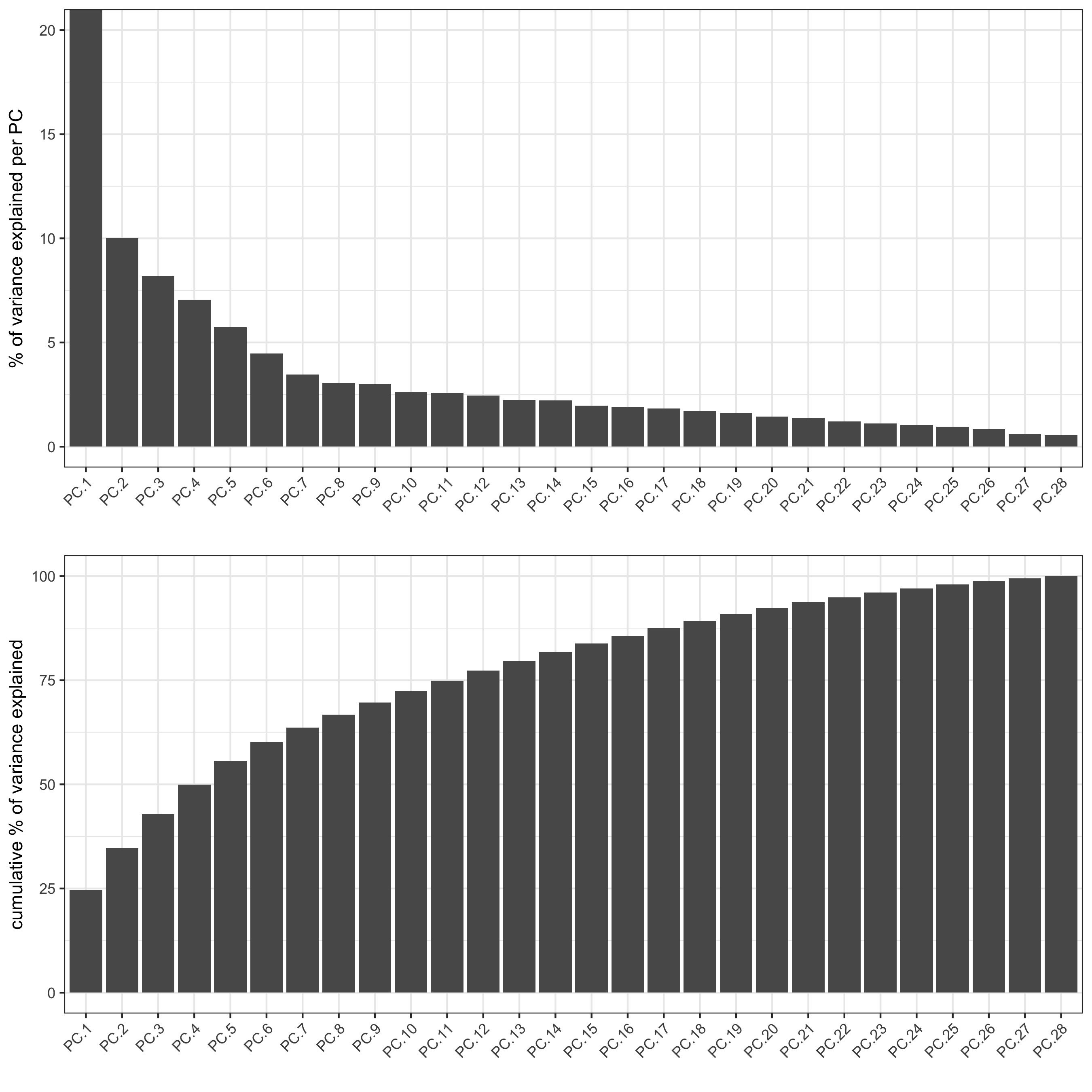
starmap_mini <- runPCA(gobject = starmap_mini, method = 'factominer')
screePlot(starmap_mini, ncp = 30,
  save_param = list(save_name = '3_a_screeplot'))
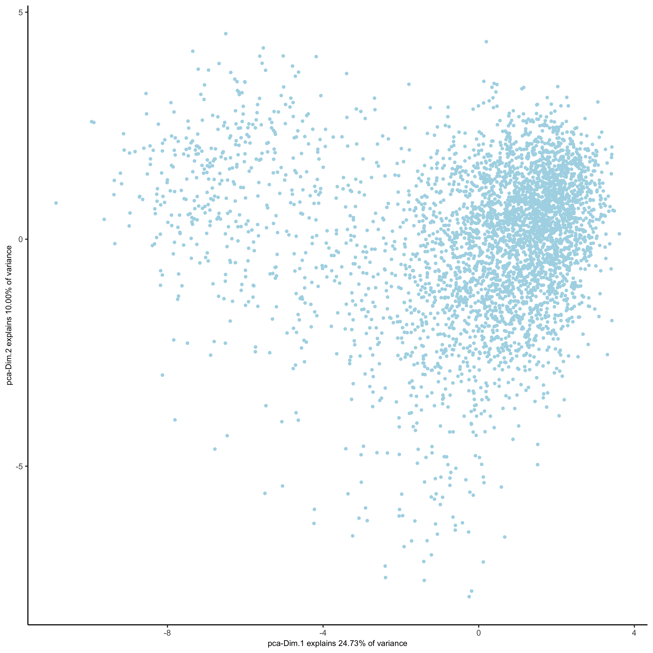
plotPCA(gobject = starmap_mini,
    save_param = list(save_name = '3_b_PCA'))
# 2D umap
starmap_mini <- runUMAP(starmap_mini, dimensions_to_use = 1:8)
plotUMAP(gobject = starmap_mini,
    save_param = list(save_name = '3_c_UMAP'))
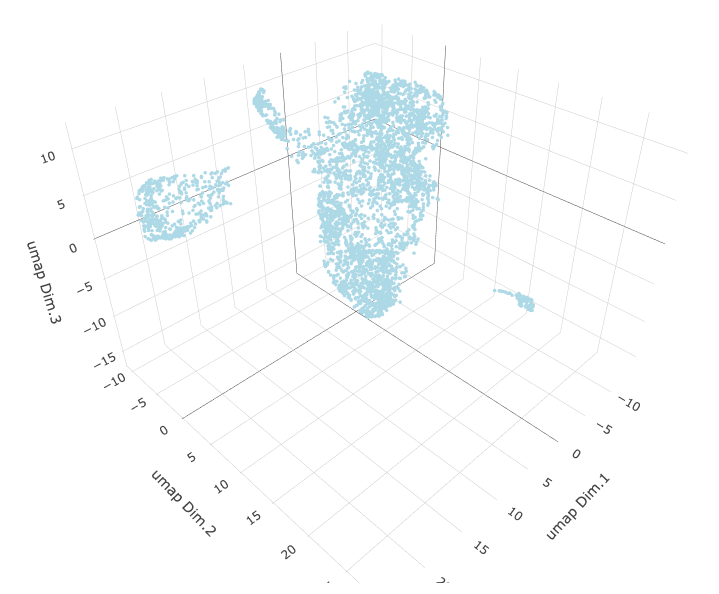
# 3D umap
starmap_mini <- runUMAP(starmap_mini, dimensions_to_use = 1:8, name = '3D_umap', n_components = 3)
plotUMAP_3D(gobject = starmap_mini, dim_reduction_name = '3D_umap',
    save_param = list(save_name = '3_d_UMAP_3D'))
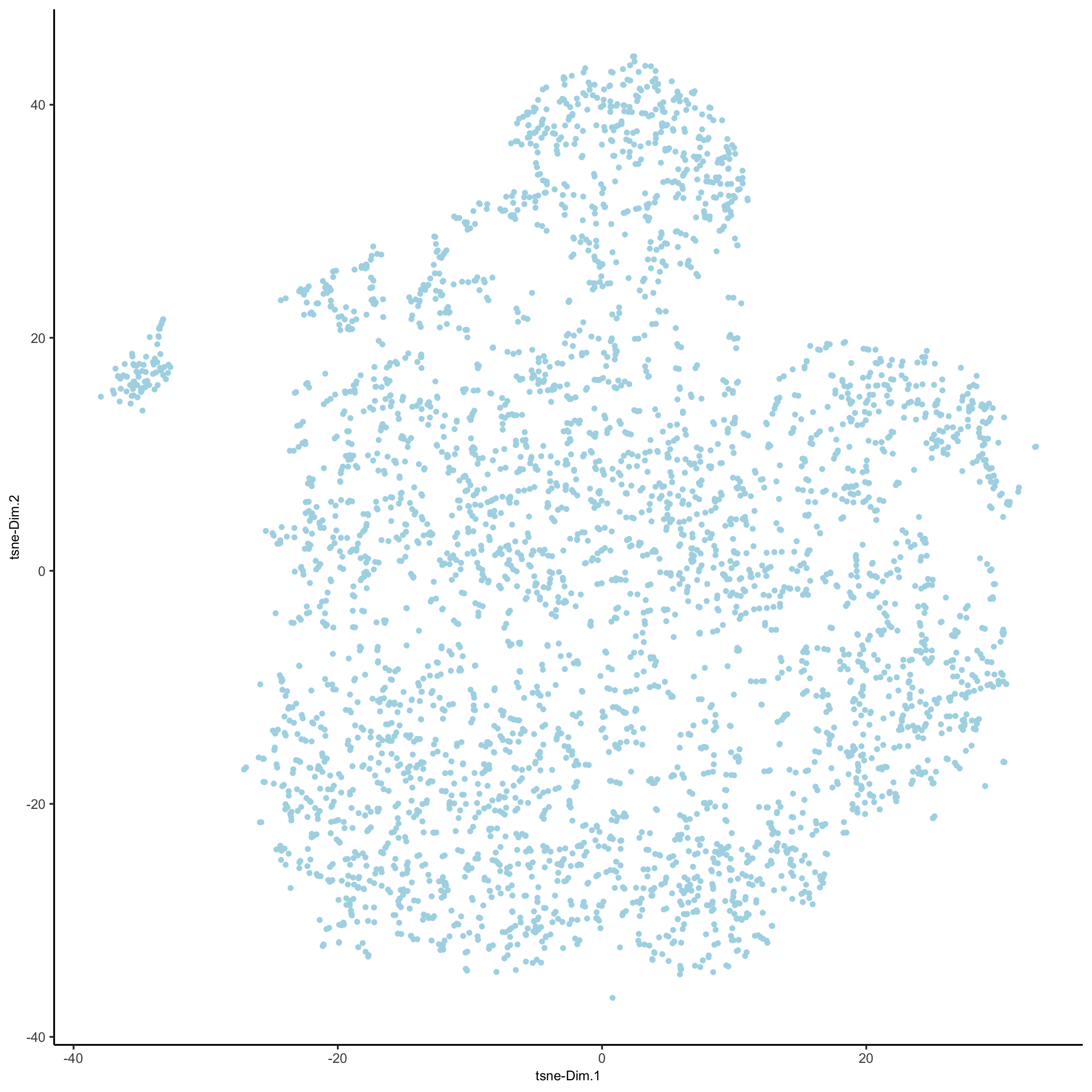
# 2D tsne
starmap_mini <- runtSNE(starmap_mini, dimensions_to_use = 1:8)
plotTSNE(gobject = starmap_mini,
    save_param = list(save_name = '3_e_TSNE'))
4. Clustering#
Create a shared (default) nearest network in PCA space (or directly on matrix)
Cluster on nearest network with Leiden or Louvan (kmeans and hclust are alternatives)
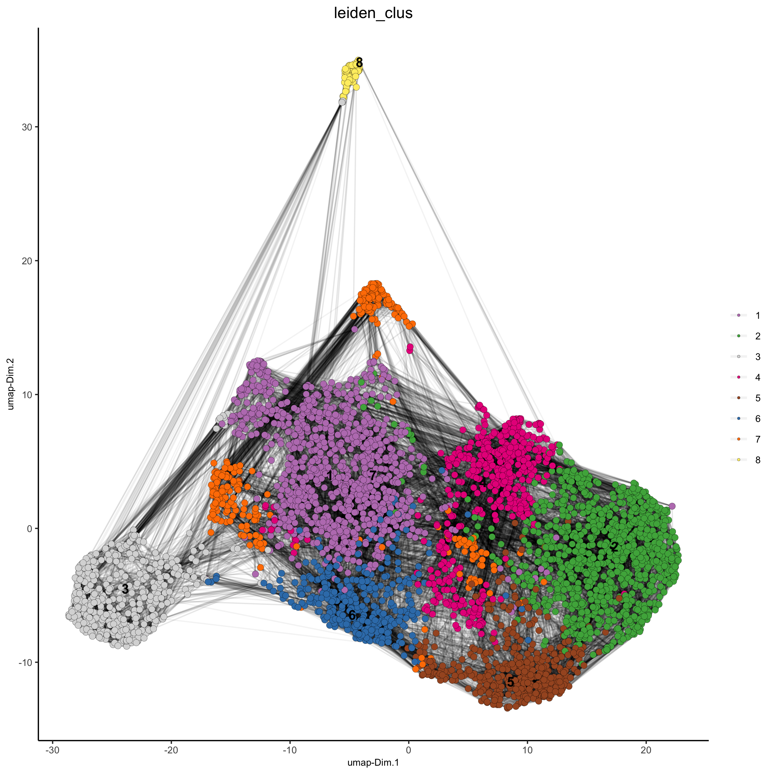
starmap_mini <- createNearestNetwork(gobject = starmap_mini, dimensions_to_use = 1:8, k = 25)
starmap_mini <- doLeidenCluster(gobject = starmap_mini, resolution = 0.5, n_iterations = 1000)

# 2D umap
plotUMAP(gobject = starmap_mini,
    cell_color = 'leiden_clus', show_NN_network = T, point_size = 2.5,
    save_param = list(save_name = '4_a_UMAP'))
# 3D umap
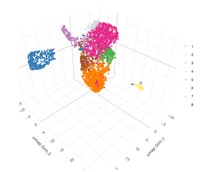
plotUMAP_3D(gobject = starmap_mini, dim_reduction_name = '3D_umap',
cell_color = 'leiden_clus',
save_param = list(save_name = '4_b_UMAP_3D'))
# 2D umap + coordinates
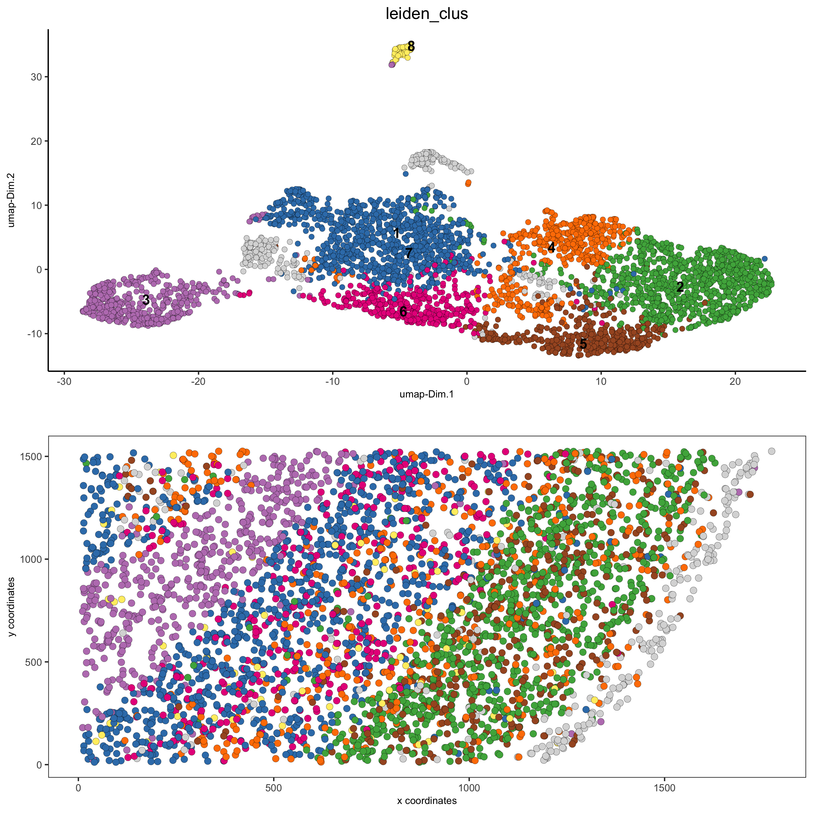
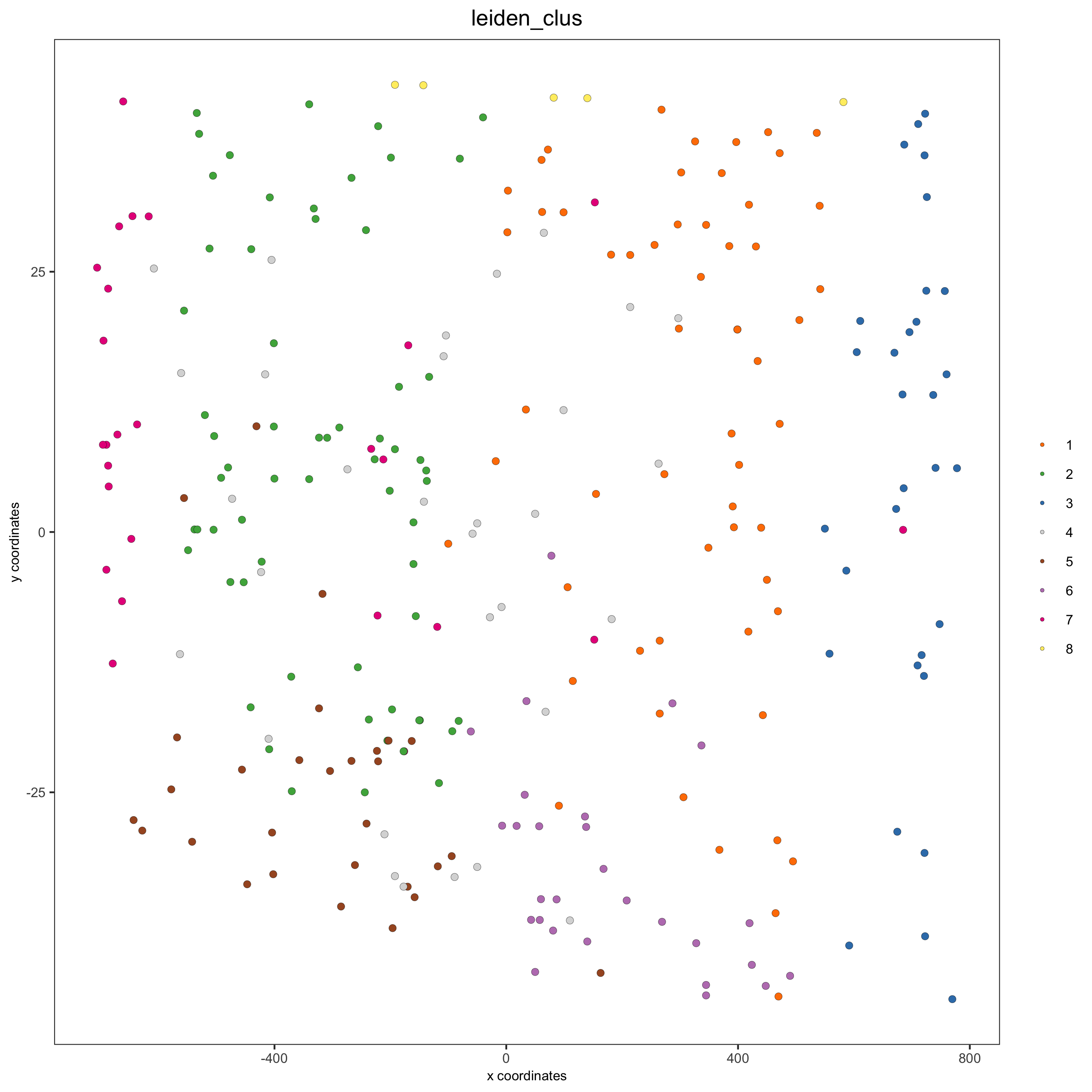
spatDimPlot(gobject = starmap_mini, cell_color = 'leiden_clus',
dim_point_size = 2, spat_point_size = 2.5,
save_param = list(save_name = '4_c_spatdimplot'))
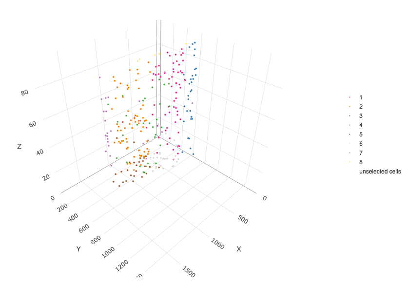
# 3D umap + coordinates
spatDimPlot3D(gobject = starmap_mini,
    cell_color = 'leiden_clus', dim_reduction_name = '3D_umap',
    save_param = list(save_name = '4_d_spatdimplot3D'))


# heatmap and dendrogram
showClusterHeatmap(gobject = starmap_mini, cluster_column = 'leiden_clus',
       save_param = list(save_name = '4_e_clusterheatmap'))

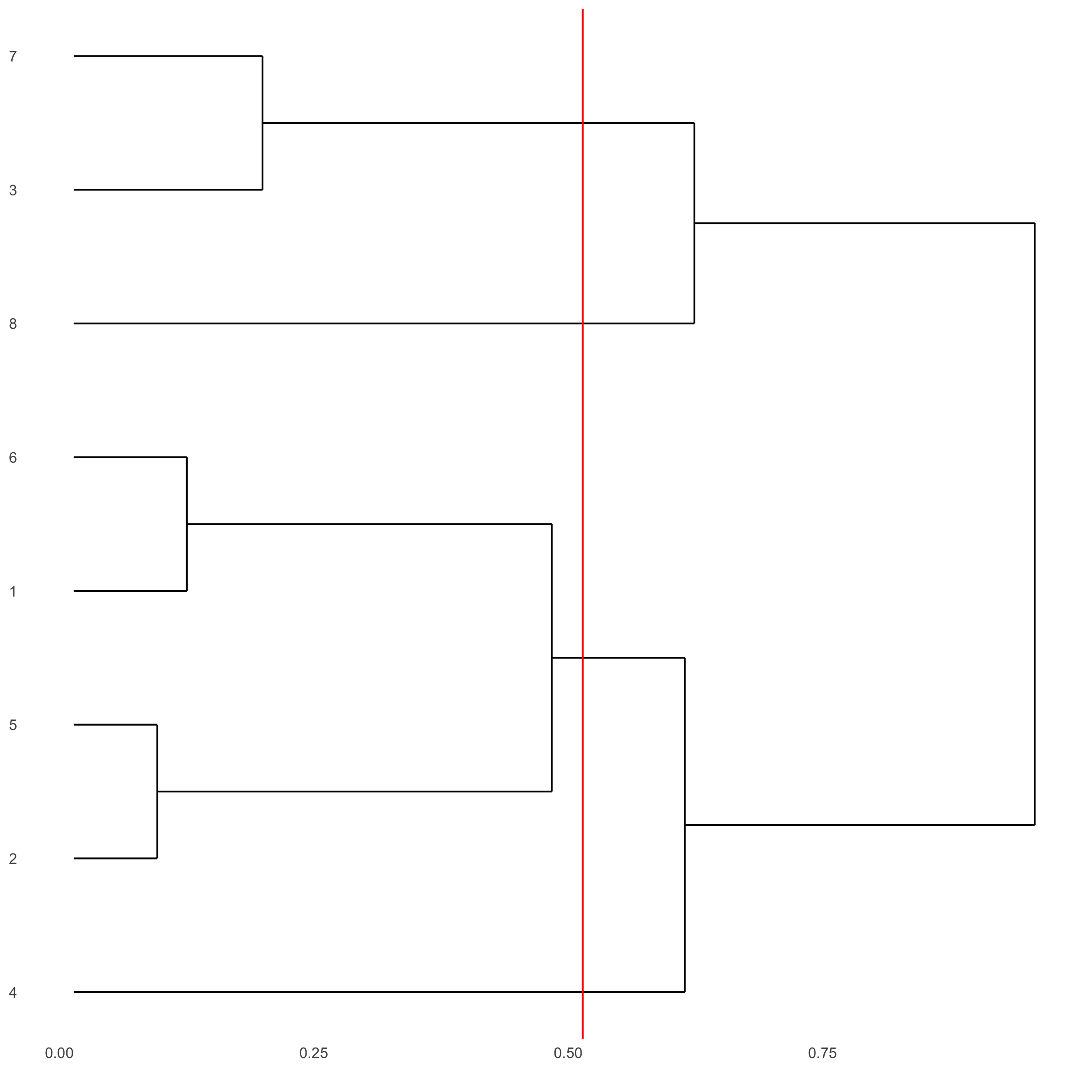
showClusterDendrogram(starmap_mini, h = 0.5, rotate = T,
          cluster_column = 'leiden_clus',
          save_param = list(save_name = '4_f_clusterdendrogram'))
5. Differential Expression#
gini_markers = findMarkers_one_vs_all(gobject = starmap_mini,
method = 'gini',
expression_values = 'normalized',
cluster_column = 'leiden_clus',
min_genes = 20,
min_expr_gini_score = 0.5,
min_det_gini_score = 0.5)
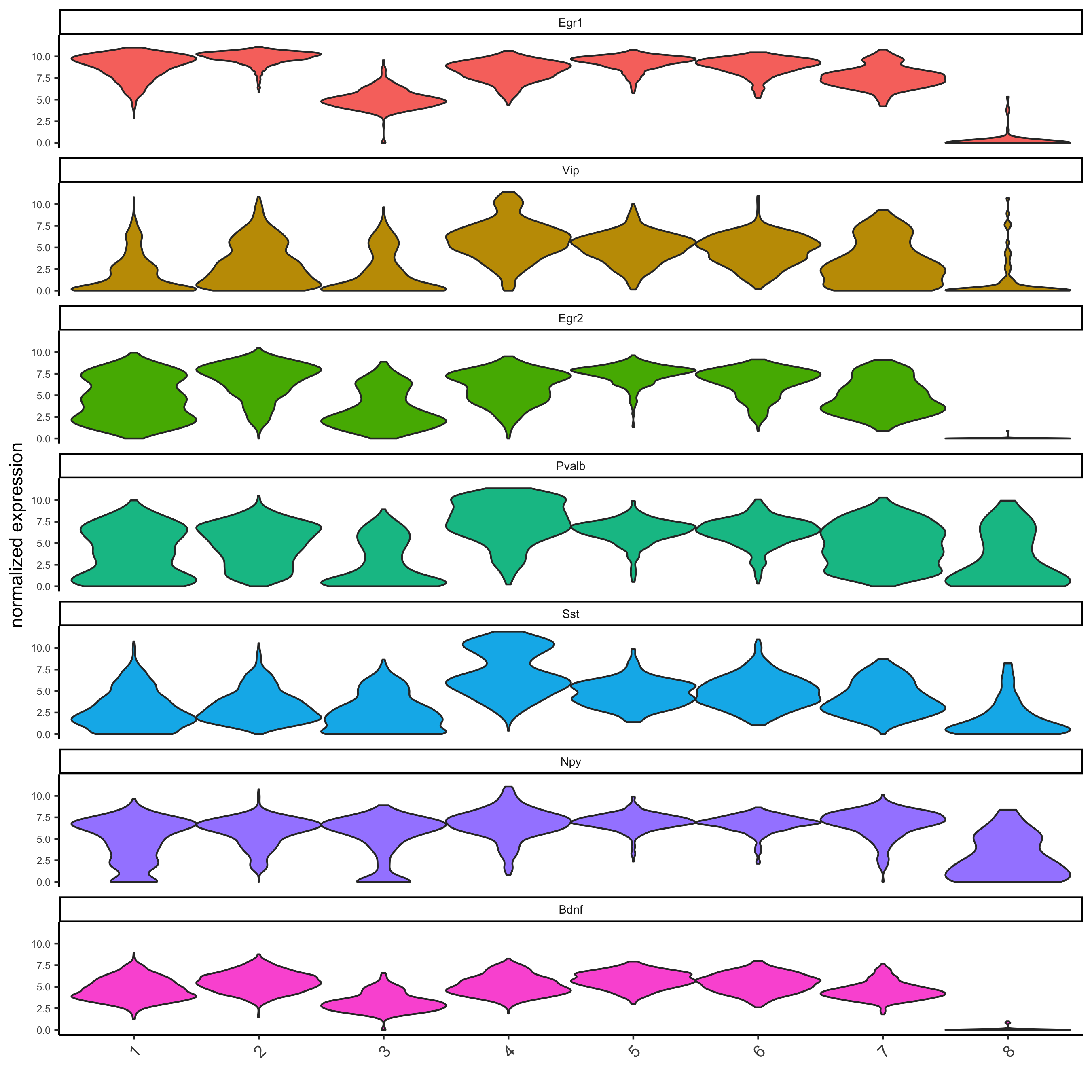
# get top 2 genes per cluster and visualize with violinplot
topgenes_gini = gini_markers[, head(.SD, 2), by = 'cluster']
violinPlot(starmap_mini, genes = topgenes_gini$genes,
cluster_column = 'leiden_clus',
save_param = list(save_name = '5_a_violinplot'))
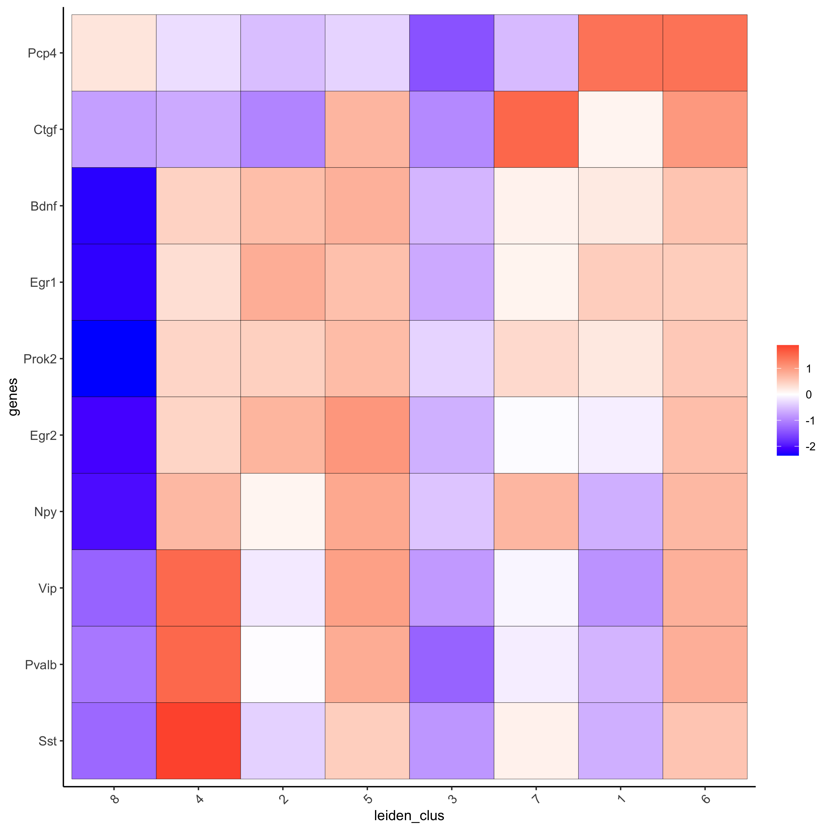
# get top 6 genes per cluster and visualize with heatmap
topgenes_gini2 = gini_markers[, head(.SD, 6), by = 'cluster']
plotMetaDataHeatmap(starmap_mini, selected_genes = topgenes_gini2$genes,
        metadata_cols = c('leiden_clus'),
        save_param = list(save_name = '5_b_metaheatmap'))
6. Cell Type#
6.1 Cell Type Annotation#
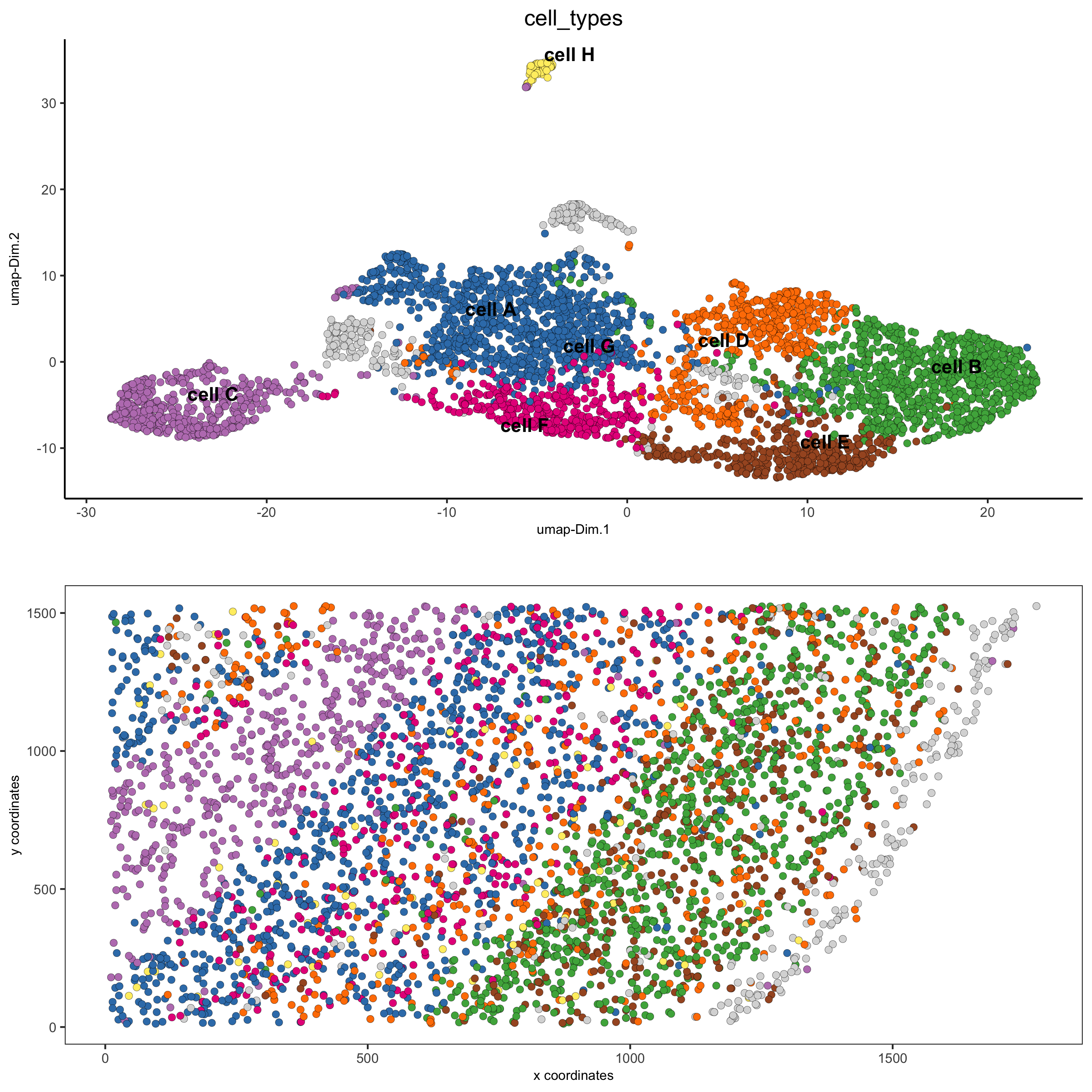
clusters_cell_types = c('cell A', 'cell B', 'cell C', 'cell D',
        'cell E', 'cell F', 'cell G', 'cell H')
names(clusters_cell_types) = 1:8
starmap_mini = annotateGiotto(gobject = starmap_mini,
              annotation_vector = clusters_cell_types,
              cluster_column = 'leiden_clus',
              name = 'cell_types')
# check new cell metadata
pDataDT(starmap_mini)

# visualize annotations
spatDimPlot(gobject = starmap_mini, cell_color = 'cell_types',
    spat_point_size = 2, dim_point_size = 2,
    save_param = list(save_name = '6_a_spatdimplot'))
6.2 Cell Type Gene Expression#
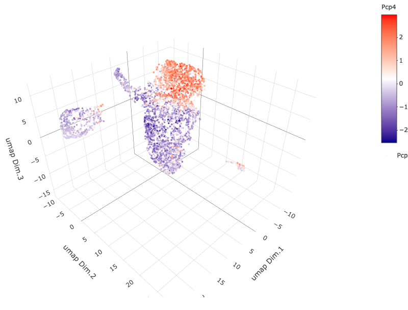
dimGenePlot3D(starmap_mini,
      dim_reduction_name = '3D_umap',
      expression_values = 'scaled',
      genes = "Pcp4",
      genes_high_color = 'red', genes_mid_color = 'white', genes_low_color = 'darkblue',
      save_param = list(save_name = '6_b_dimgeneplot'))
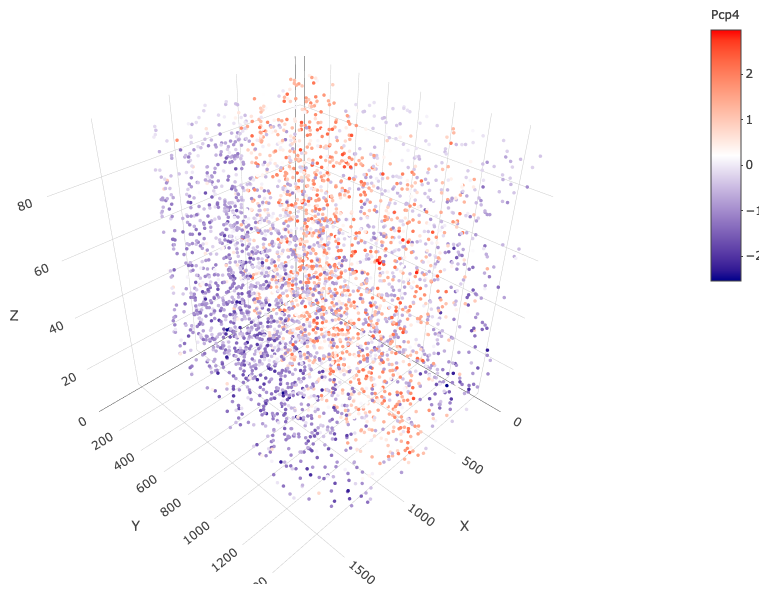
spatGenePlot3D(starmap_mini,
       expression_values = 'scaled',
       genes = "Pcp4",
       show_other_cells = F,
       genes_high_color = 'red', genes_mid_color = 'white', genes_low_color = 'darkblue',
       save_param = list(save_name = '6_c_spatgeneplot'))
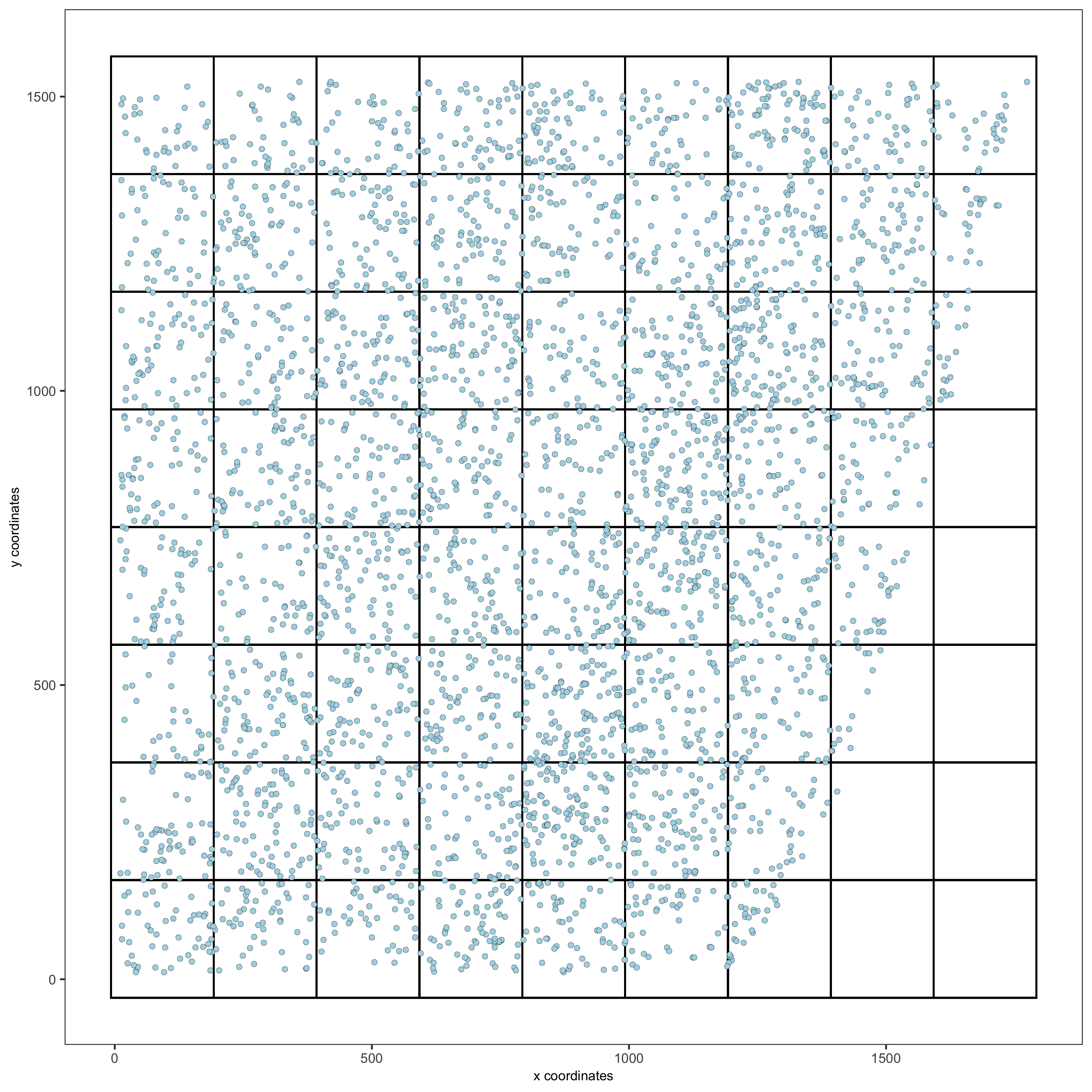
7. Spatial Grid#
Create a grid based on defined stepsizes in the x,y(,z) axes.
starmap_mini <- createSpatialGrid(gobject = starmap_mini,
              sdimx_stepsize = 200,
              sdimy_stepsize = 200,
              sdimz_stepsize = 20,
              minimum_padding = 10)
showGrids(starmap_mini)

# visualize grid
spatPlot2D(gobject = starmap_mini, show_grid = T, point_size = 1.5,
    save_param = list(save_name = '7_a_spatplot'))
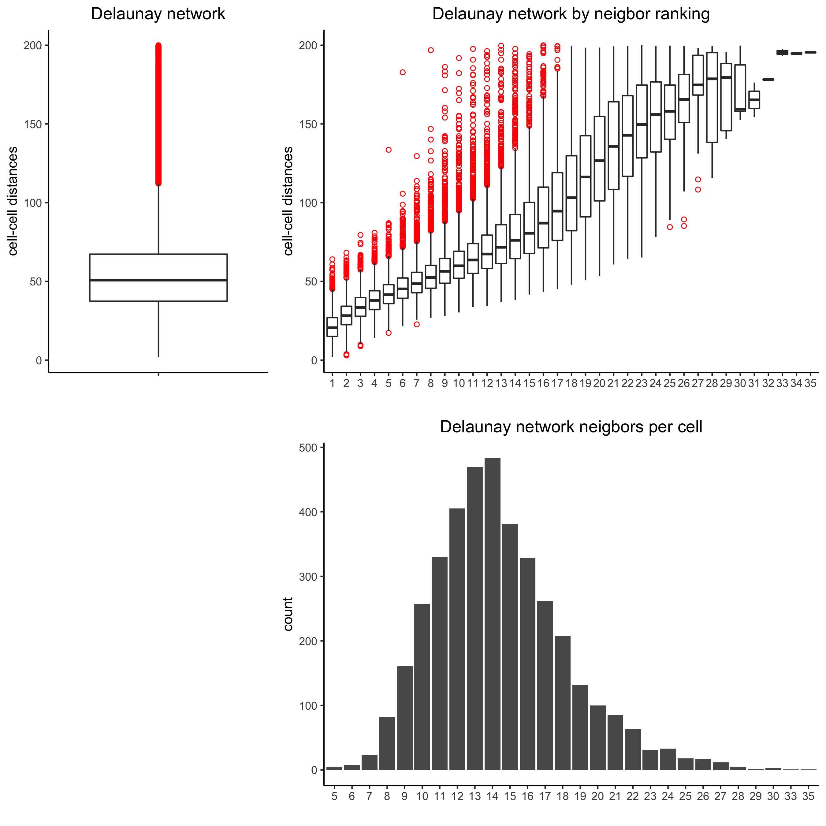
8. Spatial Network#
Only the method = delaunayn_geometry can make 3D Delaunay networks. This requires the package geometry to be installed.
Visualize information about the default Delaunay network
Create a spatial Delaunay network (default)
Create a spatial kNN network
plotStatDelaunayNetwork(gobject = starmap_mini, maximum_distance = 200,
        method = 'delaunayn_geometry',
        save_param = list(save_name = '8_aa_delnetwork'))
starmap_mini = createSpatialNetwork(gobject = starmap_mini, minimum_k = 2,
maximum_distance_delaunay = 200,
method = 'Delaunay',
delaunay_method = 'delaunayn_geometry')
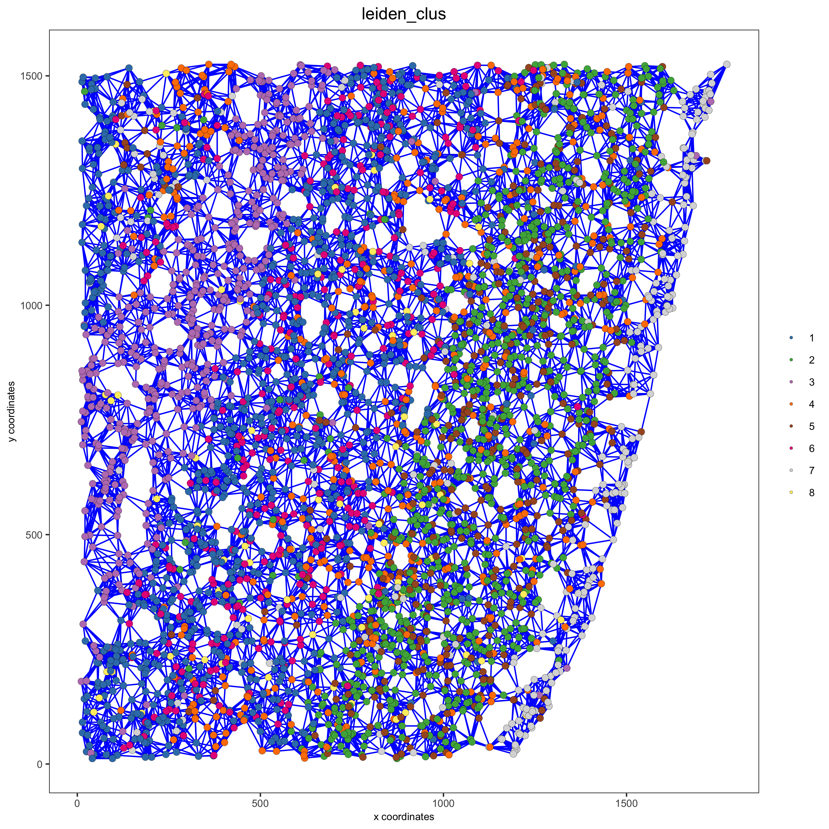
starmap_mini = createSpatialNetwork(gobject = starmap_mini, minimum_k = 2,
method = 'kNN', k = 10)
showNetworks(starmap_mini)
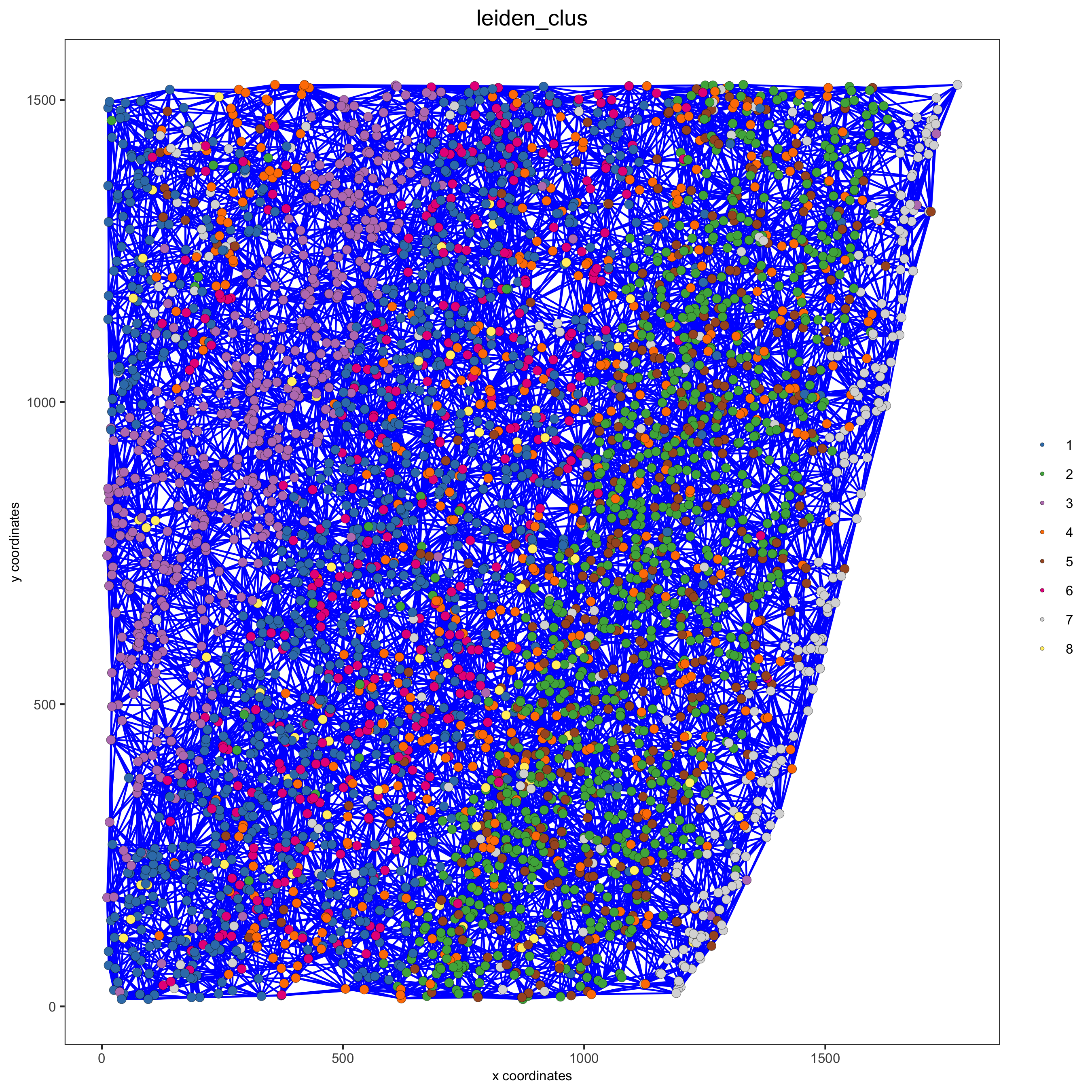
# visualize the two different spatial networks
spatPlot(gobject = starmap_mini, show_network = T,
network_color = 'blue', spatial_network_name = 'Delaunay_network',
point_size = 2.5, cell_color = 'leiden_clus',
save_param = list(save_name = '8_a_spatplot'))
spatPlot(gobject = starmap_mini, show_network = T,
    network_color = 'blue', spatial_network_name = 'kNN_network',
    point_size = 2.5, cell_color = 'leiden_clus',
    save_param = list(save_name = '8_b_spatplot'))
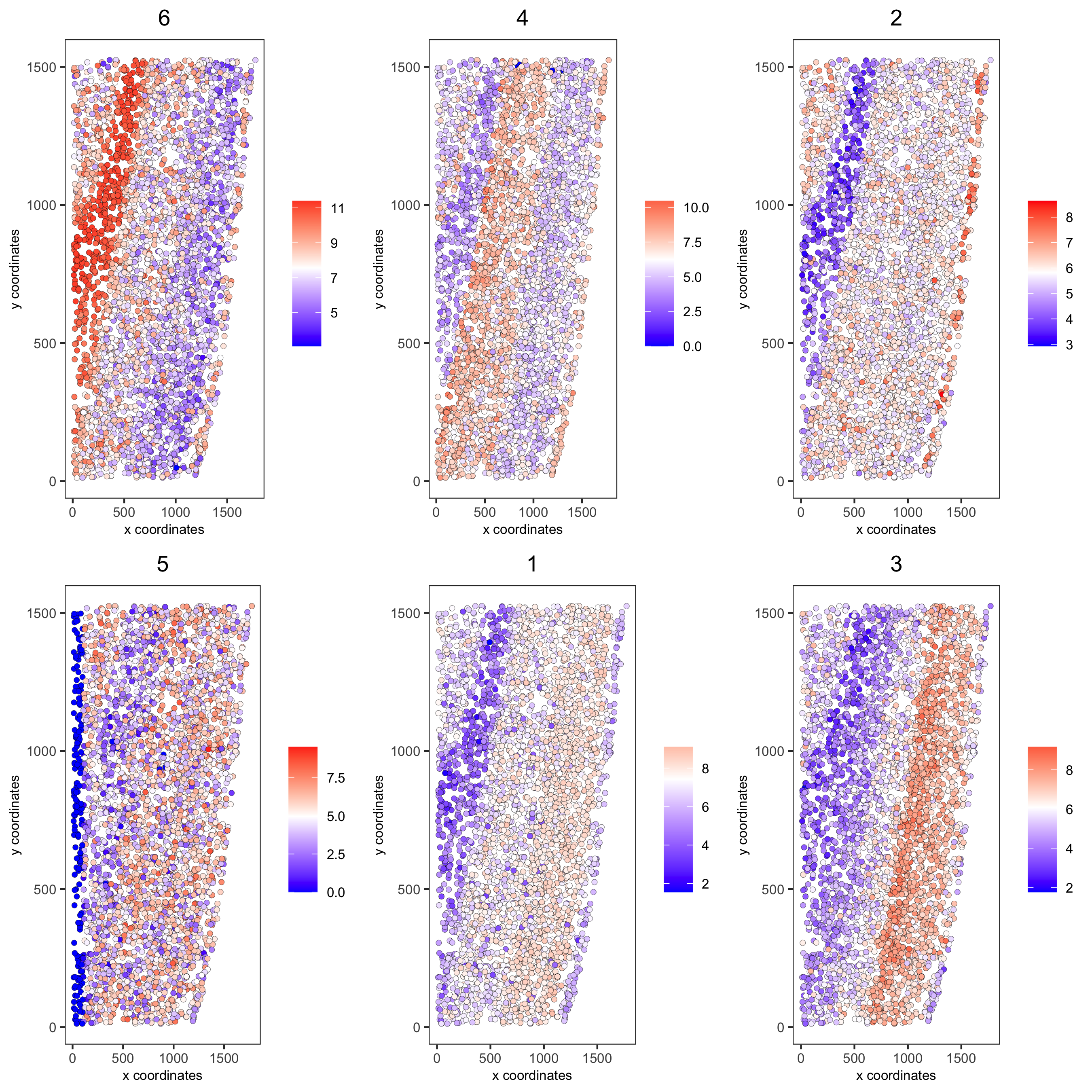
9. Spatial Genes#
Identify spatial genes with 3 different methods:
binSpect with kmeans binarization (default)
binSpect with rank binarization
silhouetteRank
Visualize top 4 genes per method.
km_spatialgenes = binSpect(starmap_mini)
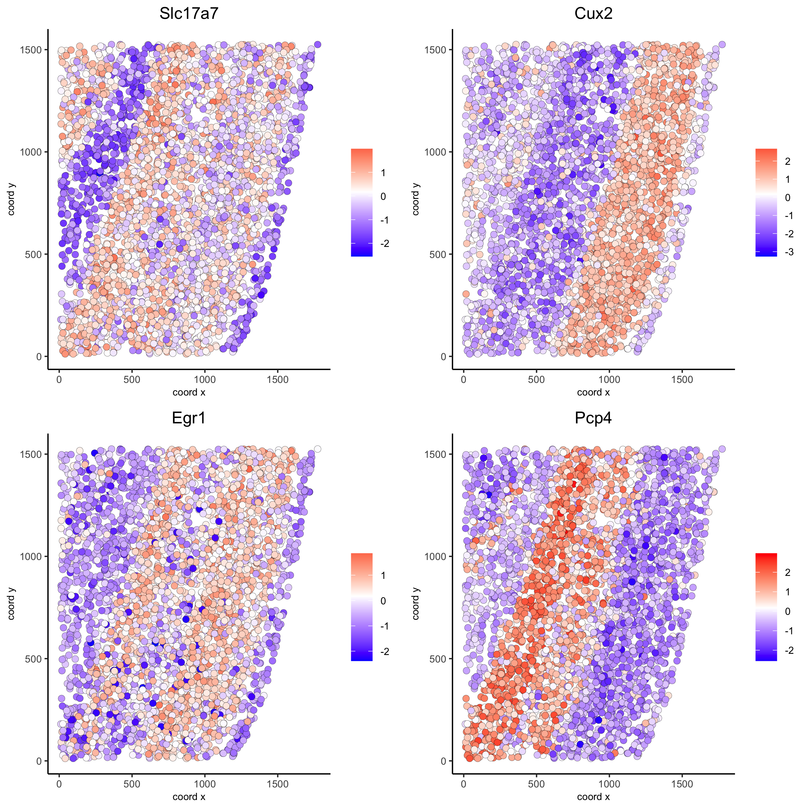
spatGenePlot(starmap_mini, expression_values = 'scaled',
genes = km_spatialgenes[1:4]$genes,
point_shape = 'border', point_border_stroke = 0.1,
show_network = F, network_color = 'lightgrey', point_size = 2.5,
cow_n_col = 2,
save_param = list(save_name = '9_a_spatgeneplot'))
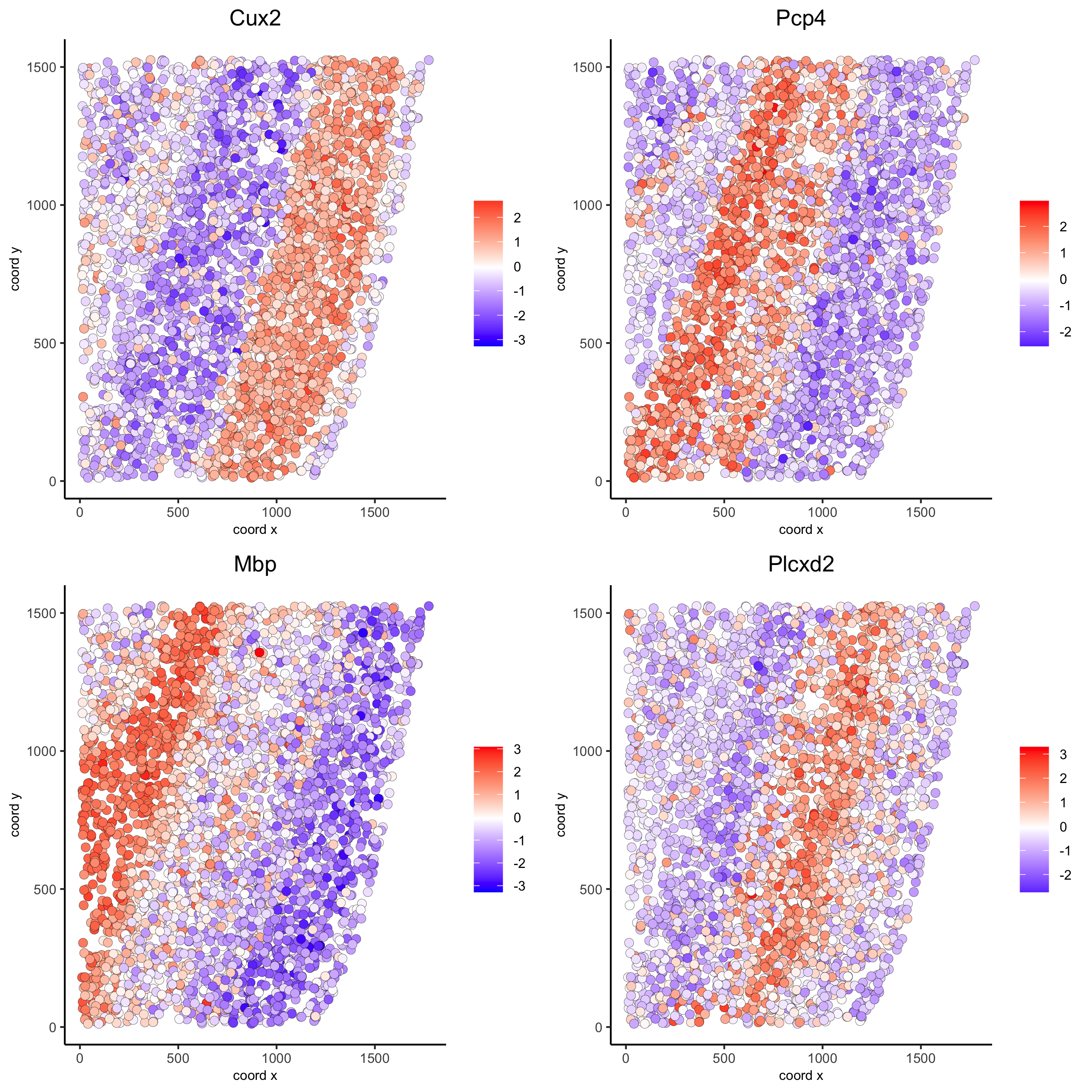
rank_spatialgenes = binSpect(starmap_mini, bin_method = 'rank')
spatGenePlot(starmap_mini, expression_values = 'scaled',
    genes = rank_spatialgenes[1:4]$genes,
    point_shape = 'border', point_border_stroke = 0.1,
    show_network = F, network_color = 'lightgrey', point_size = 2.5,
    cow_n_col = 2,
    save_param = list(save_name = '9_b_spatgeneplot'))
silh_spatialgenes = silhouetteRank(gobject = starmap_mini) # TODO: suppress print output
spatGenePlot(starmap_mini, expression_values = 'scaled',
    genes = silh_spatialgenes[1:4]$genes,
    point_shape = 'border', point_border_stroke = 0.1,
    show_network = F, network_color = 'lightgrey', point_size = 2.5,
    cow_n_col = 2,
    save_param = list(save_name = '9_c_spatgeneplot'))
10. Spatial Co-Expression Patterns#
Identify robust spatial co-expression patterns using the spatial network or grid and a subset of individual spatial genes.
10.1 Calculate spatial correlation scores#
# 1. calculate spatial correlation scores
ext_spatial_genes = km_spatialgenes[1:20]$genes
spat_cor_netw_DT = detectSpatialCorGenes(starmap_mini,
                 method = 'network',
                 spatial_network_name = 'Delaunay_network',
                 subset_genes = ext_spatial_genes)
10.2. Cluster correlation scores#
# 2. cluster correlation scores
spat_cor_netw_DT = clusterSpatialCorGenes(spat_cor_netw_DT,
name = 'spat_netw_clus', k = 6)
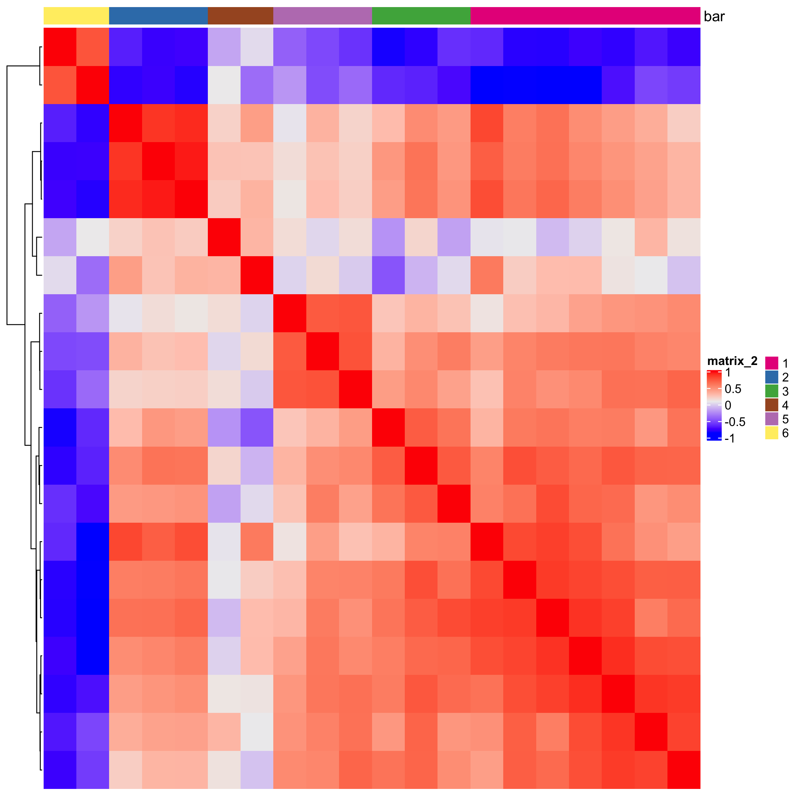
heatmSpatialCorGenes(starmap_mini, spatCorObject = spat_cor_netw_DT,
use_clus_name = 'spat_netw_clus',
save_param = list(save_name = '10_a_heatmspatcor', units = 'in'))
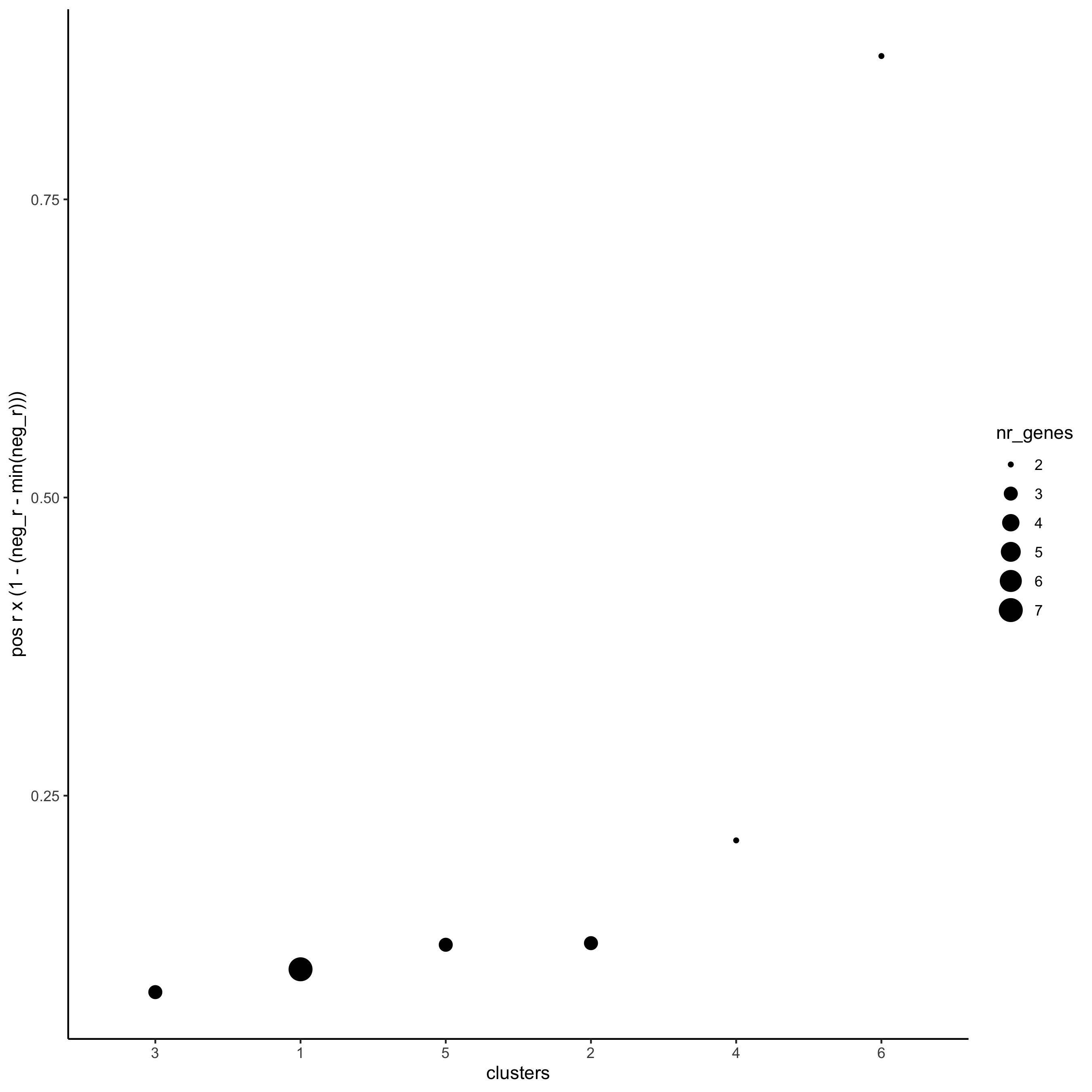
netw_ranks = rankSpatialCorGroups(starmap_mini,
              spatCorObject = spat_cor_netw_DT,
              use_clus_name = 'spat_netw_clus',
              save_param = list(save_name = '10_b_rankcorgroup'))
top_netw_spat_cluster = showSpatialCorGenes(spat_cor_netw_DT,
                    use_clus_name = 'spat_netw_clus',
                    selected_clusters = 6,
                    show_top_genes = 1)

cluster_genes_DT = showSpatialCorGenes(spat_cor_netw_DT,
                   use_clus_name = 'spat_netw_clus',
                   show_top_genes = 1)
cluster_genes = cluster_genes_DT$clus; names(cluster_genes) = cluster_genes_DT$gene_ID


starmap_mini = createMetagenes(starmap_mini,
               gene_clusters = cluster_genes,
               name = 'cluster_metagene')
spatCellPlot(starmap_mini,
    spat_enr_names = 'cluster_metagene',
    cell_annotation_values = netw_ranks$clusters,
    point_size = 1.5, cow_n_col = 3,
    save_param = list(save_name = '10_c_spatcellplot'))
11. Spatial HMRF Domains#
hmrf_folder = paste0(temp_dir,'/','11_HMRF/')
if(!file.exists(hmrf_folder)) dir.create(hmrf_folder, recursive = T)

# perform hmrf
my_spatial_genes = km_spatialgenes[1:20]$genes
HMRF_spatial_genes = doHMRF(gobject = starmap_mini,
            expression_values = 'scaled',
            spatial_genes = my_spatial_genes,
            spatial_network_name = 'Delaunay_network',
            k = 6,
            betas = c(10,2,2),
            output_folder = paste0(hmrf_folder, '/', 'Spatial_genes/SG_top20_k6_scaled'))

# check and select hmrf
for(i in seq(10, 14, by = 2)) {
viewHMRFresults2D(gobject = starmap_mini,
        HMRFoutput = HMRF_spatial_genes,
        k = 6, betas_to_view = i,
        point_size = 2)
}

starmap_mini = addHMRF(gobject = starmap_mini,
        HMRFoutput = HMRF_spatial_genes,
        k = 6, betas_to_add = c(12),
        hmrf_name = 'HMRF')

# visualize selected hmrf result
giotto_colors = Giotto:::getDistinctColors(6)
names(giotto_colors) = 1:6
spatPlot(gobject = starmap_mini, cell_color = 'HMRF_k6_b.12',
    point_size = 3, coord_fix_ratio = 1, cell_color_code = giotto_colors,
    save_param = list(save_name = '11_a_spatplot'))
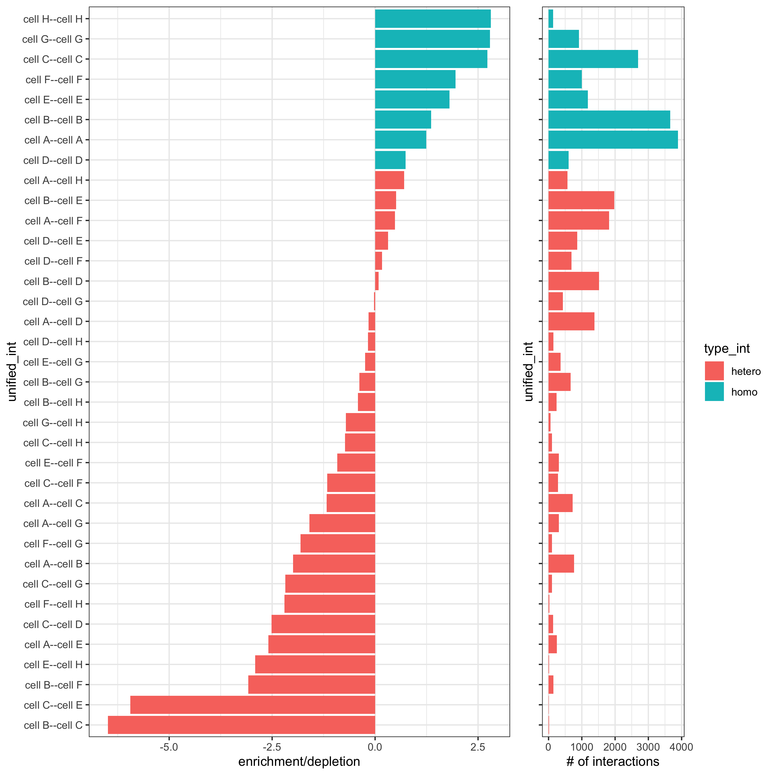
12. Cell Neighborhood: Cell-Type / Cell-Type Interactions#
set.seed(seed = 2841)
cell_proximities = cellProximityEnrichment(gobject = starmap_mini,
                   cluster_column = 'cell_types',
                   spatial_network_name = 'Delaunay_network',
                   adjust_method = 'fdr',
                   number_of_simulations = 1000)
# barplot
cellProximityBarplot(gobject = starmap_mini,
         CPscore = cell_proximities,
         min_orig_ints = 2, min_sim_ints = 2, p_val = 0.5,
         save_param = list(save_name = '12_a_barplot'))
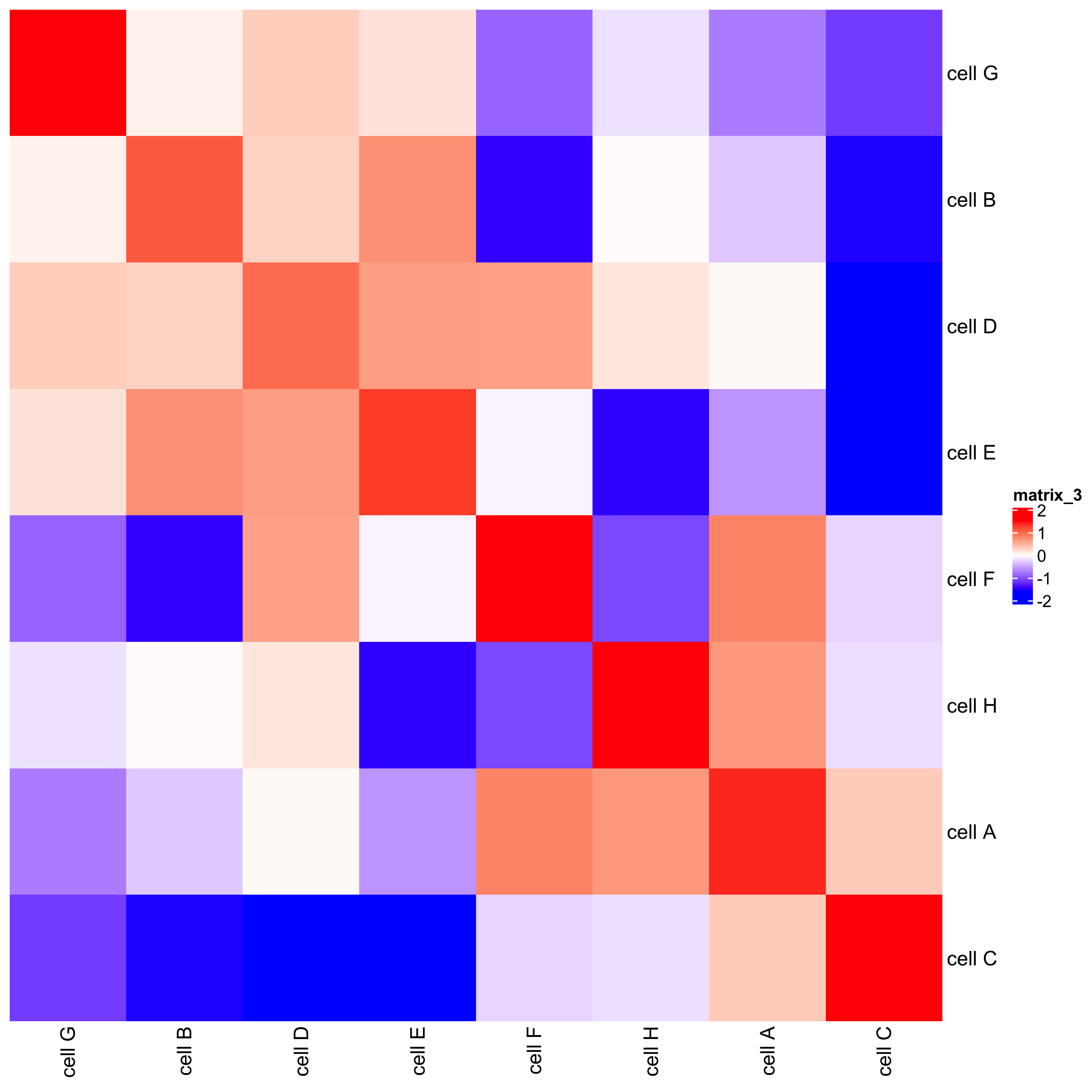
## heatmap
cellProximityHeatmap(gobject = starmap_mini, CPscore = cell_proximities,
         order_cell_types = T, scale = T,
         color_breaks = c(-1.5, 0, 1.5),
         color_names = c('blue', 'white', 'red'),
         save_param = list(save_name = '12_b_heatmap', units = 'in'))
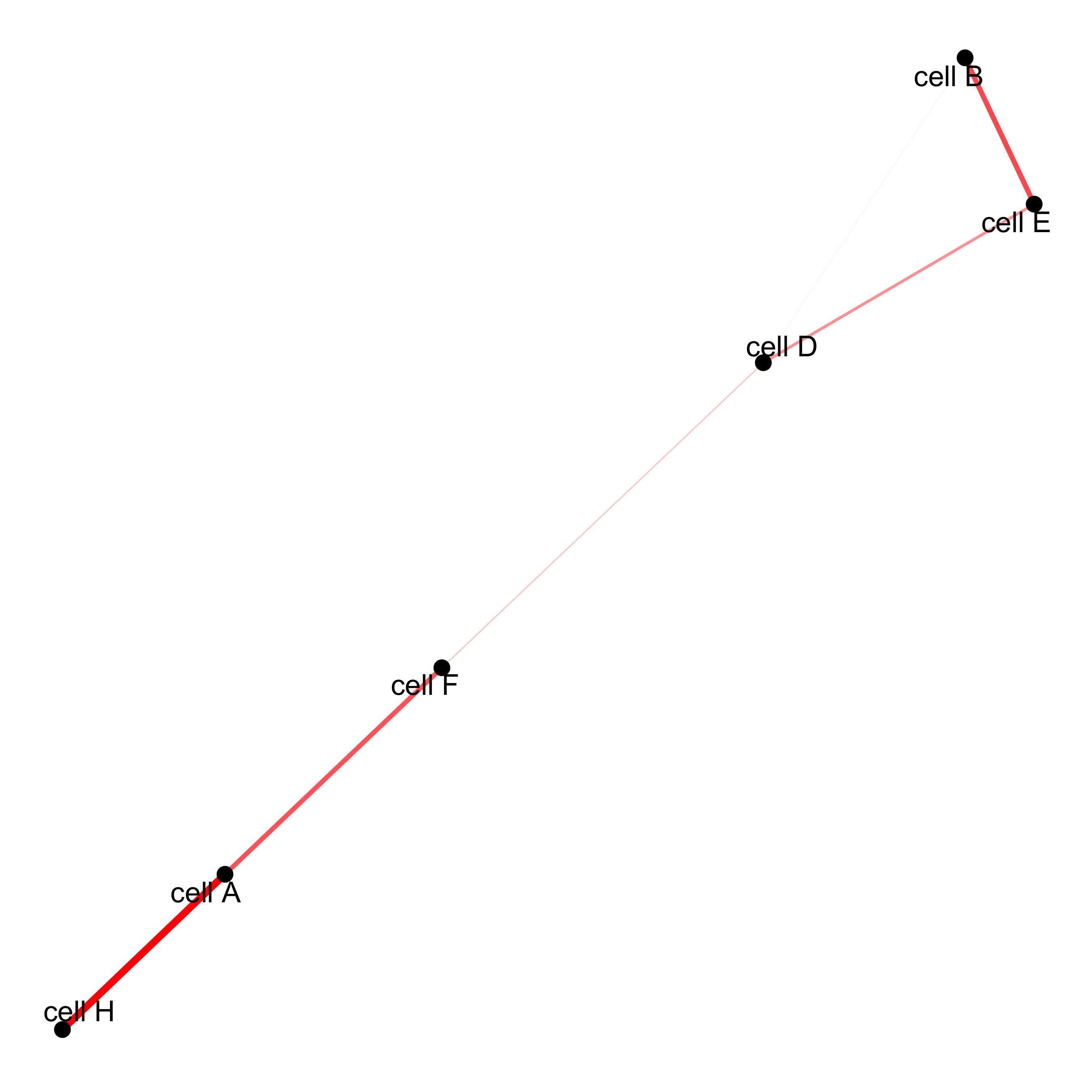
# network
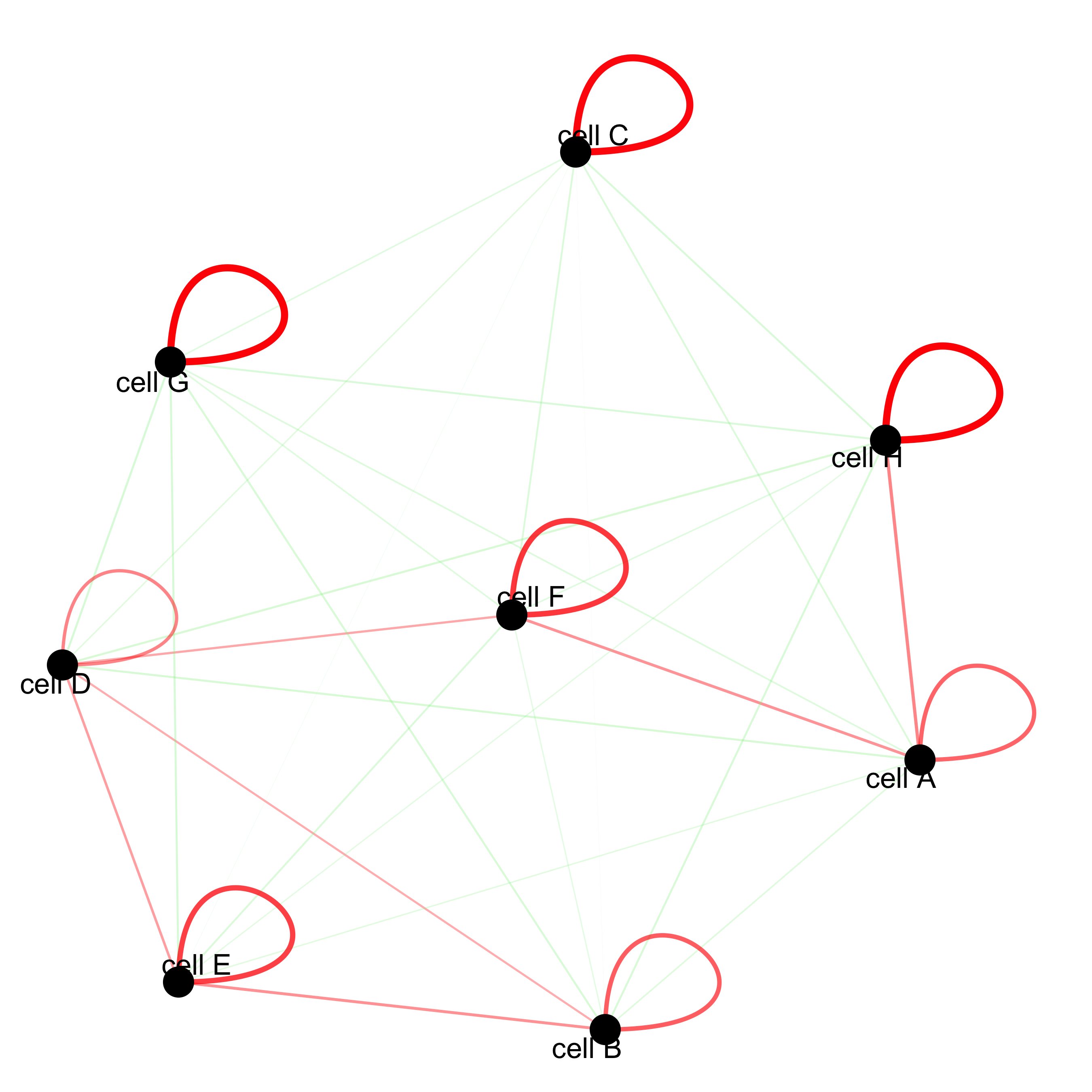
cellProximityNetwork(gobject = starmap_mini, CPscore = cell_proximities,
remove_self_edges = T, only_show_enrichment_edges = T,
save_param = list(save_name = '12_c_network'))
# network with self-edges
cellProximityNetwork(gobject = starmap_mini, CPscore = cell_proximities,
        remove_self_edges = F, self_loop_strength = 0.3,
        only_show_enrichment_edges = F,
        rescale_edge_weights = T,
        node_size = 8,
        edge_weight_range_depletion = c(1, 2),
        edge_weight_range_enrichment = c(2,5),
        save_param = list(save_name = '12_d_network'))
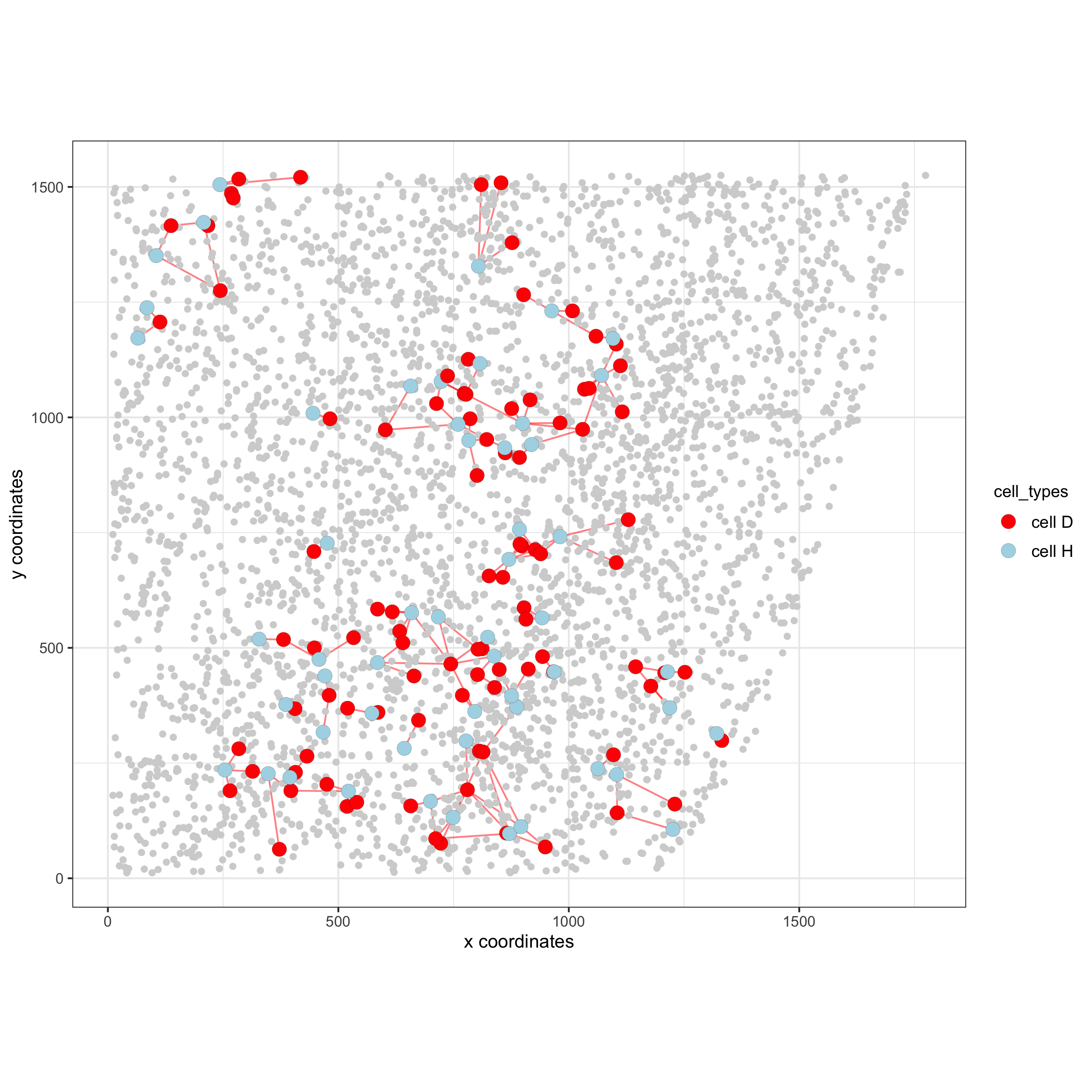
12.1 Visualization of Specific Cell Types#
Option 1#
pDataDT(starmap_mini)
# Option 1
spec_interaction = "cell D--cell H" # needs to be in alphabetic order! first D, then H
cellProximitySpatPlot2D(gobject = starmap_mini,
            interaction_name = spec_interaction,
            show_network = T,
            cluster_column = 'cell_types',
            cell_color = 'cell_types',
            cell_color_code = c('cell H' = 'lightblue', 'cell D' = 'red'),
            point_size_select = 4, point_size_other = 2,
            save_param = list(save_name = '12_e_cellproximity'))
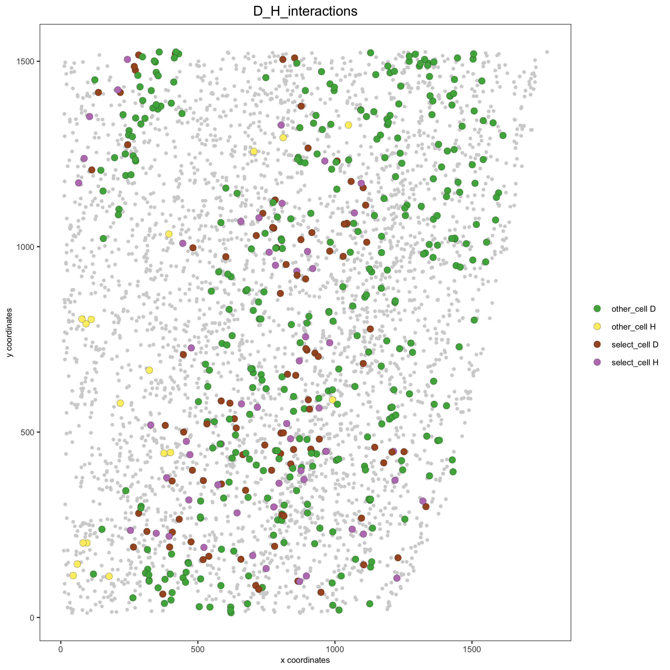
Option 2#
# Option 2: create additional metadata
starmap_mini = addCellIntMetadata(starmap_mini,
             spatial_network = 'Delaunay_network',
             cluster_column = 'cell_types',
             cell_interaction = spec_interaction,
             name = 'D_H_interactions')
spatPlot(starmap_mini, cell_color = 'D_H_interactions', legend_symbol_size = 3,
    select_cell_groups =  c('other_cell D', 'other_cell H', 'select_cell D', 'select_cell H'),
    save_param = list(save_name = '12_e_spatplot'))
13. 2D cross sections from 3D object#
# create cross section
starmap_mini = createCrossSection(starmap_mini,
method="equation",
equation=c(0,1,0,600),
extend_ratio = 0.6)
# show cross section
insertCrossSectionSpatPlot3D(starmap_mini, cell_color = 'leiden_clus',
axis_scale = 'cube',
point_size = 2,
save_param = list(save_name = '13_a_insertcross'))
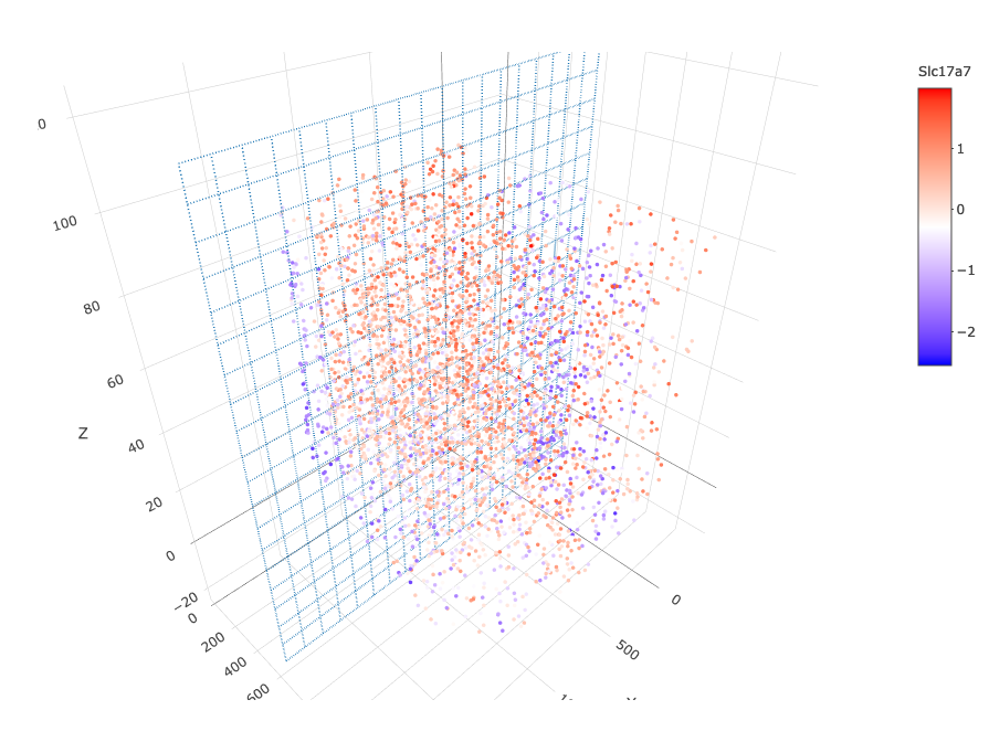
insertCrossSectionGenePlot3D(starmap_mini, expression_values = 'scaled',
axis_scale = "cube",
genes = "Slc17a7",
save_param = list(save_name = '13_b_insertcrossgene'))
# for cell annotation
crossSectionPlot(starmap_mini,
        point_size = 2, point_shape = "border",
        cell_color = "leiden_clus",
        save_param = list(save_name = '13_c_crossplot'))
crossSectionPlot3D(starmap_mini,
       point_size = 2, cell_color = "leiden_clus",
       axis_scale = "cube",
       save_param = list(save_name = '13_c_crossplot3D'))
# for gene expression
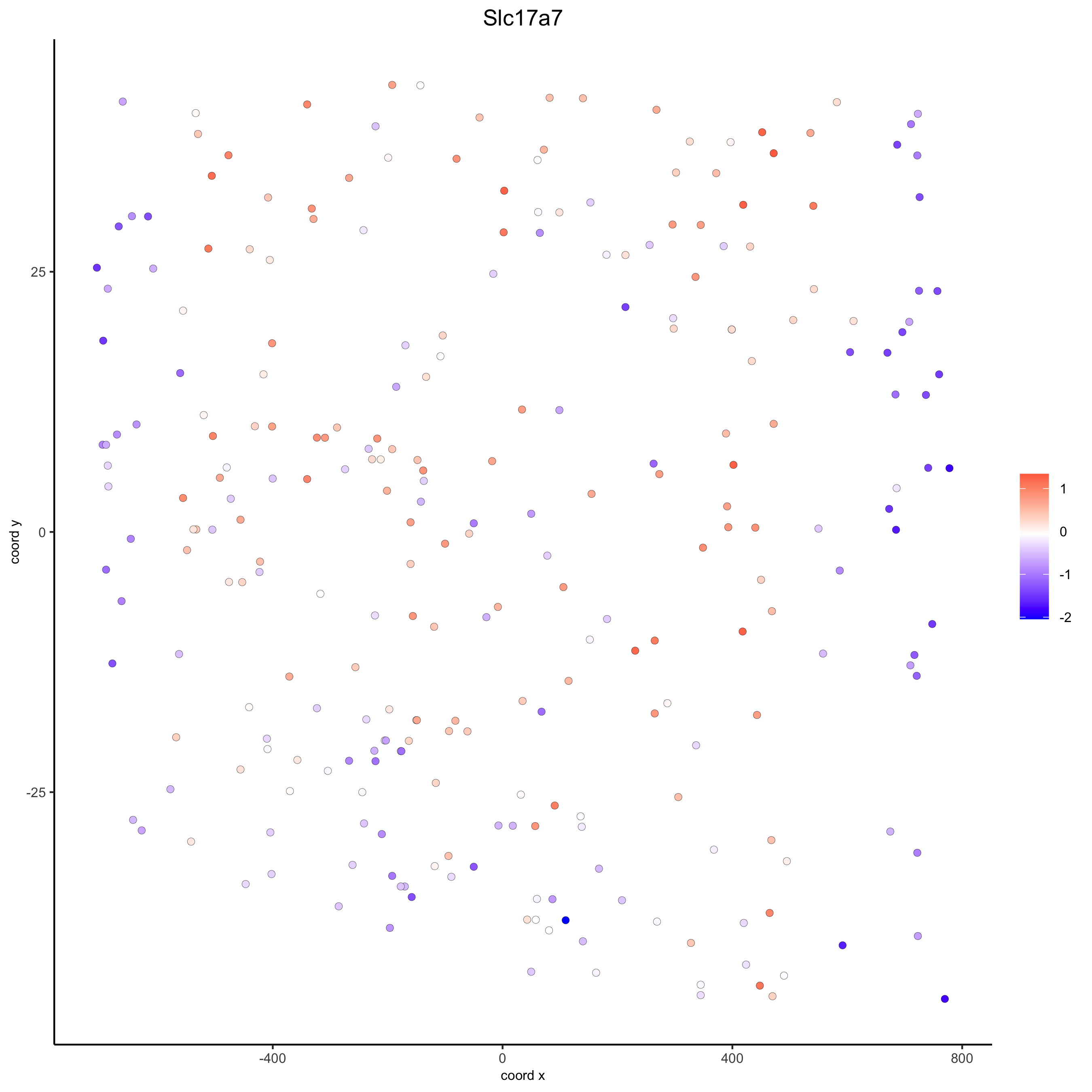
crossSectionGenePlot(starmap_mini,
genes = "Slc17a7",
point_size = 2,
point_shape = "border",
cow_n_col = 1.5,
expression_values = 'scaled',
save_param = list(save_name = '13_d_crossgeneplot'))
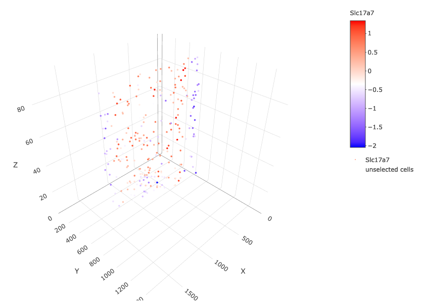
crossSectionGenePlot3D(starmap_mini,
           point_size = 2,
           genes = c("Slc17a7"),
           expression_values = 'scaled',
           save_param = list(save_name = '13_e_crossgeneplot3D'))
14. Export Giotto Analyzer to Viewer#
viewer_folder = paste0(temp_dir, '/', 'Mouse_cortex_viewer')

# select annotations, reductions and expression values to view in Giotto Viewer
exportGiottoViewer(gobject = starmap_mini, output_directory = viewer_folder,
       factor_annotations = c('cell_types',
                  'leiden_clus',
                  'HMRF_k6_b.12'),
       numeric_annotations = 'total_expr',
       dim_reductions = c('umap'),
       dim_reduction_names = c('umap'),
       expression_values = 'scaled',
       expression_rounding = 3,
       overwrite_dir = T)