Adding and Working with Images in Giotto: How to Work with Background Images?
All spatial visualization functions in the Giotto toolbox can be overlaid on a background image. This allows you to visualize your results on top of the original tissue image. We provide multiple ways of adding and modifying figures in Giotto.
There are 3 things to consider:
1. How to add an image to a Giotto object?
createGiottoVisiumObject can be used directly for a visium 10X dataset
createGiottoImage can be used to create a Giotto image object from a magick image object
addGiottoImage this add a Giotto image to your Giotto object
updateGiottoImage this helps to adjust the alignment of your image with your results
2. How to modify an image (i.e. change the background color)?
estimateImageBg function to estimate the background color of your Giotto or magick image
changeImageBg function to change the background color of your image
plotGiottoImage function to plot an image by itself
3. How to show these images with your spatial plots?
showGiottoImageNames: this tells you which giotto image(s) are part of your giotto object
Each spatial plotting function has the following 3 parameters:
show_image = TRUE or FALSE, to show a background image or not
image_name = name of associated Giotto image to use for the background image (option 1)
gimage = a giotto image object to use (option 2)
addGiottoImageToSpatPlot to test your giotto images you can use this function to them to spatPlot result
Here we process the Visium Kidney dataset to illustrate all of the different and flexible ways to deal with images using Giotto:
1. Create Giotto Object
Here we use the wrapper function createGiottoVisiumObject to create a Giotto object for a 10X Visium dataset, which includes a png image.
library(Giotto)

visium_kidney = createGiottoVisiumObject(visium_dir = '/path/to/Visium_data/Kidney_data',
                     png_name = 'tissue_lowres_image.png', gene_column_index = 2)
2. Align Plot
The image plot and the Giotto results are not always perfectly aligned. This step just needs to be done once.
# output from Giotto
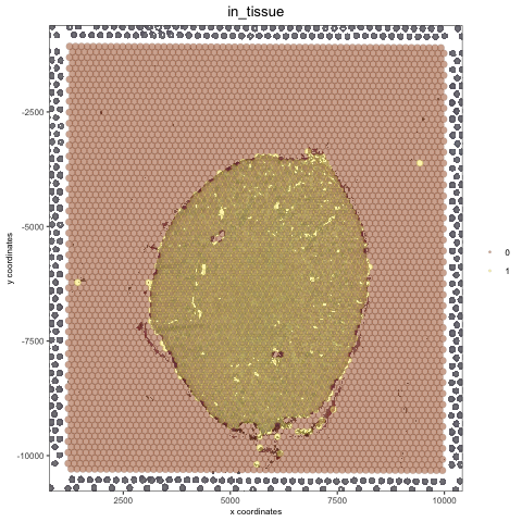
spatPlot(gobject = visium_kidney, cell_color = 'in_tissue', point_alpha = 0.5)
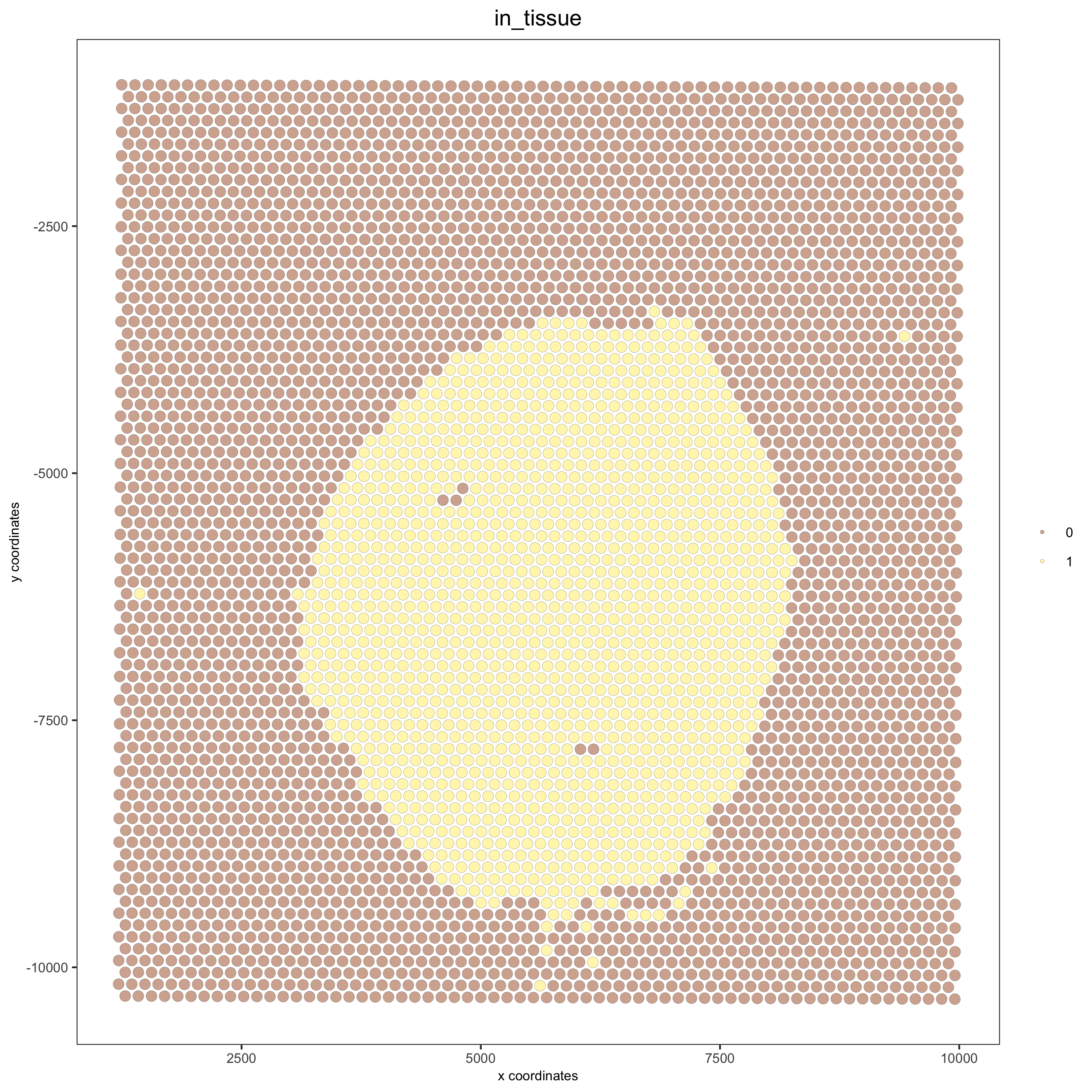
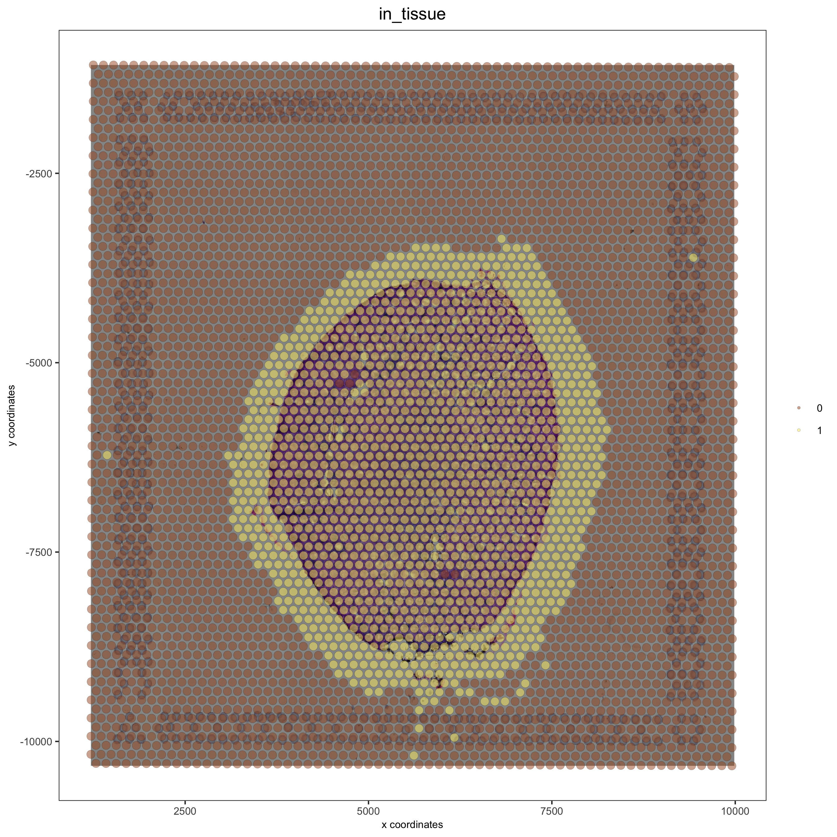
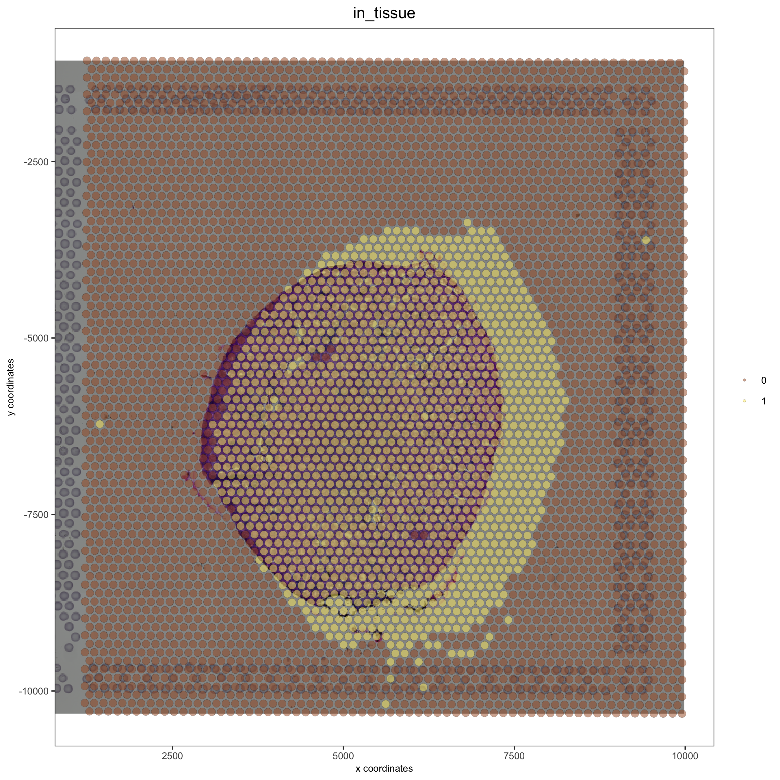
# problem: image is not perfectly aligned
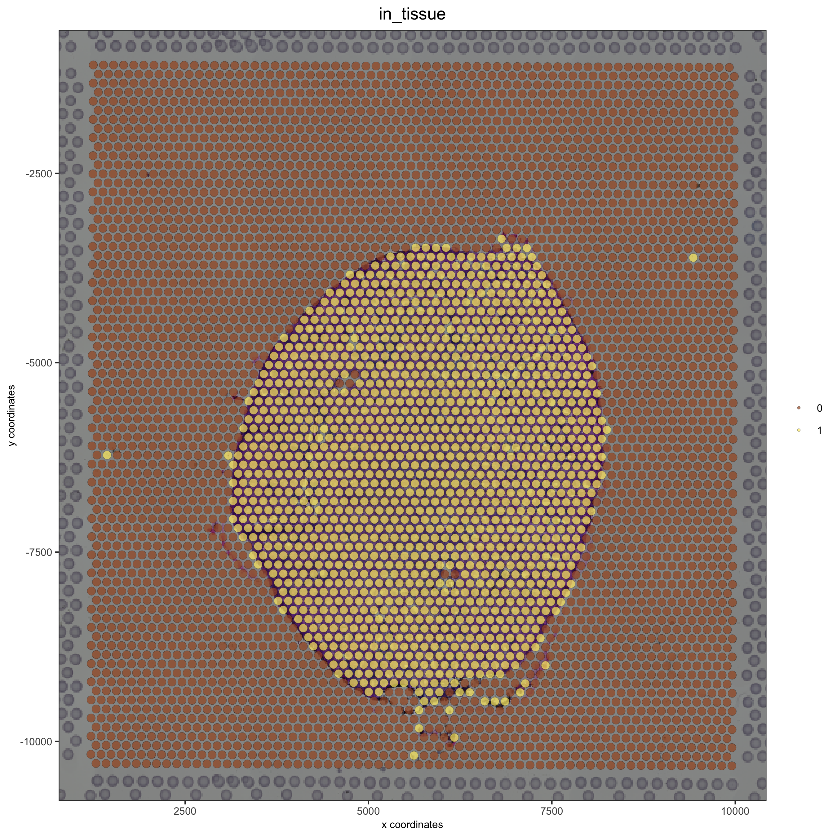
spatPlot(gobject = visium_kidney, cell_color = 'in_tissue', show_image = T, point_alpha = 0.5)

Adjust the x and y minima and maxima to align the image and the giotto output results:
Alignment Insights
X and Y Control
We can use updateGiottoImage and spatPlot in an iterative manner to see how changing the x and y minima and maxima affect the image.
xmax_adj and xmin_adj: adjust the x location (in data coordinates) giving horizontal location of raster (offset values) ymax_adj and ymin_adj: adjust the y location (in data coordinates) giving vertical location of raster (offset values)
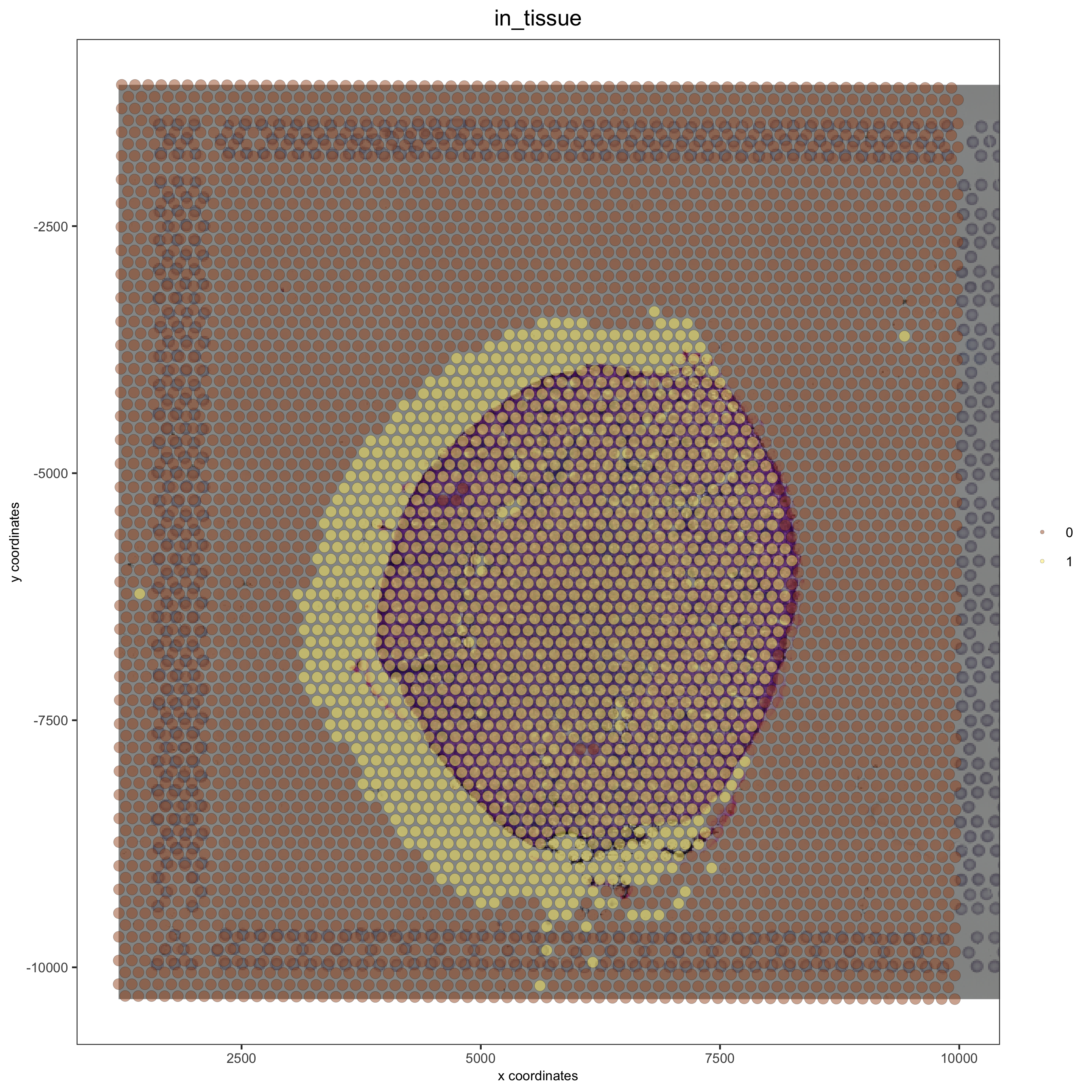
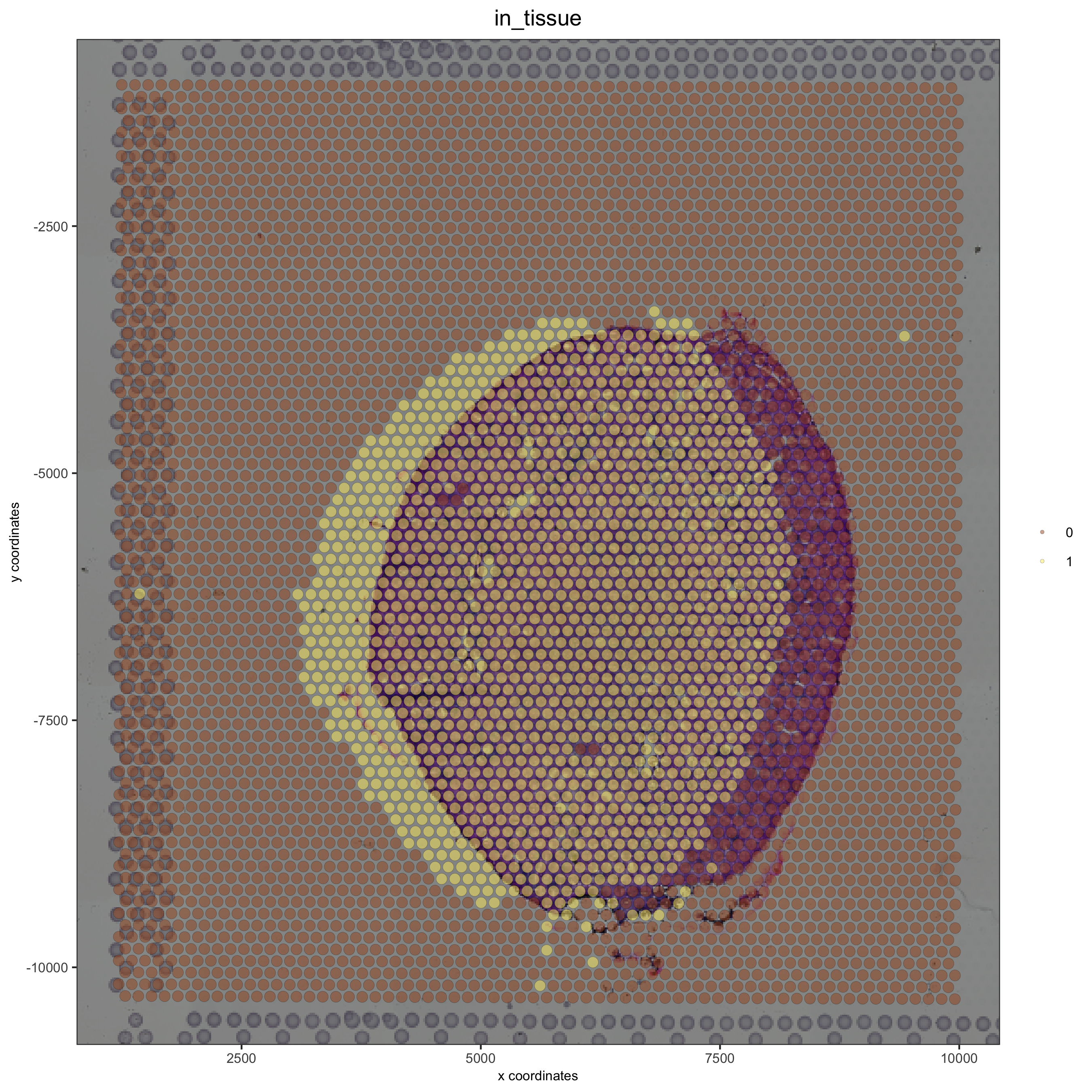
Without adjustment:
## no adjustment
visium_kidney = updateGiottoImage(visium_kidney, image_name = 'image',
               xmax_adj = 0, xmin_adj = 0,
                ymax_adj = 0, ymin_adj = 0)

spatPlot(gobject = visium_kidney, cell_color = 'in_tissue', show_image = T, point_alpha = 0.5)
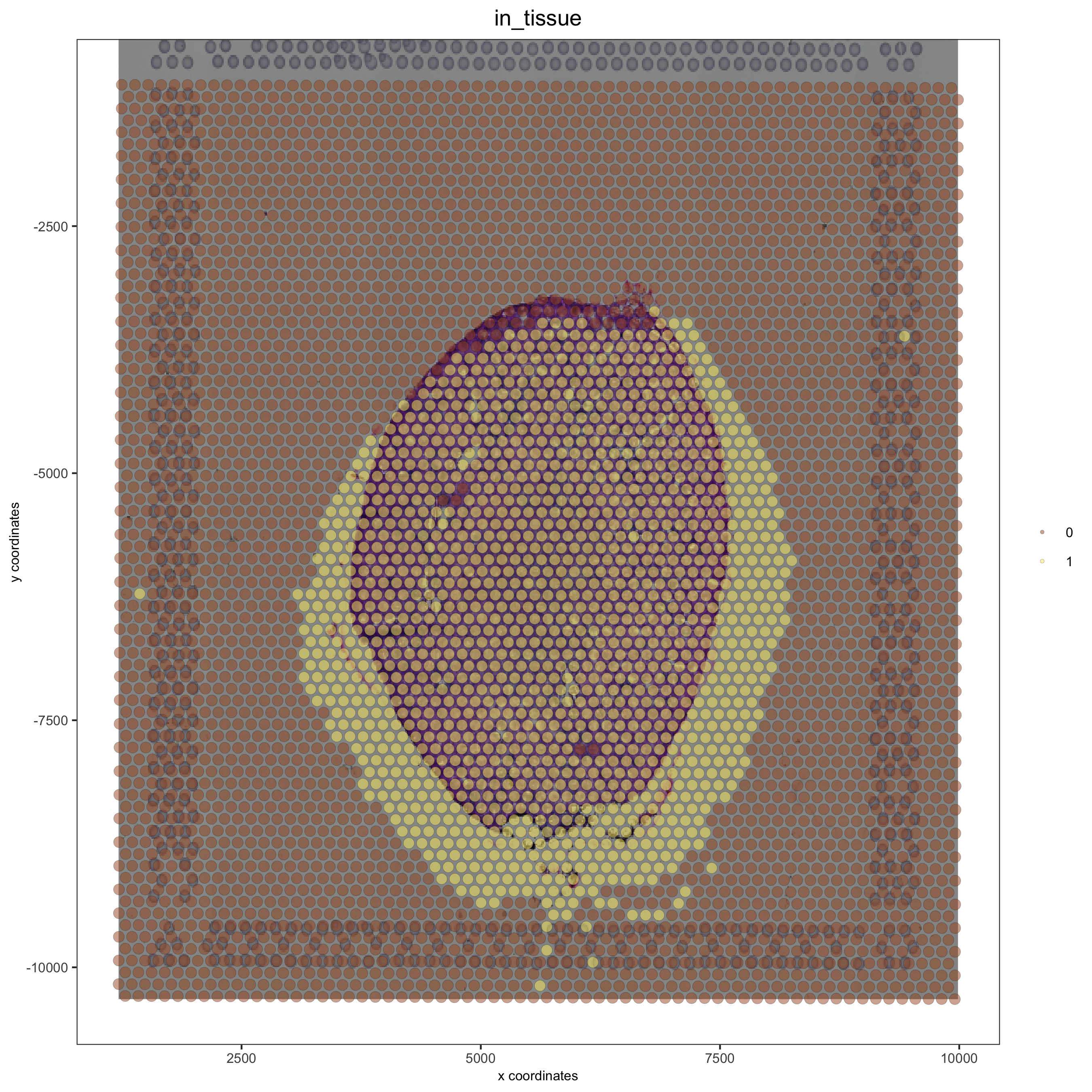
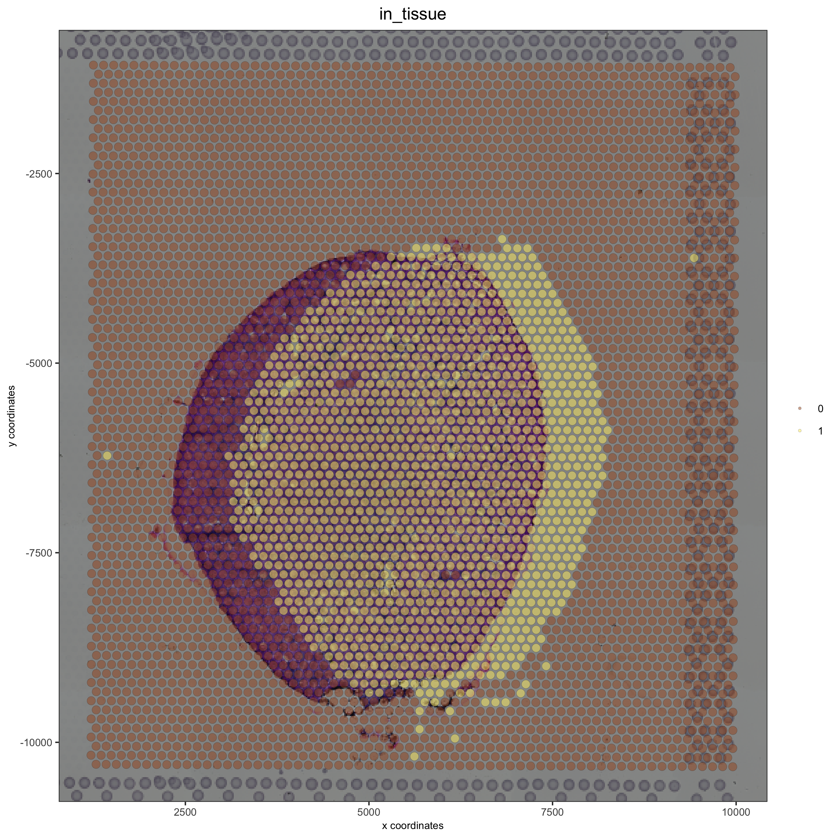
Right Adjustment –> with xmax_adj:
## adjust the image to right side with xmax_adj
visium_kidney = updateGiottoImage(visium_kidney, image_name = 'image',
                xmax_adj = 1000, xmin_adj = 0,
                ymax_adj = 0, ymin_adj = 0)

spatPlot(gobject = visium_kidney, cell_color = 'in_tissue', show_image = T, point_alpha = 0.5)
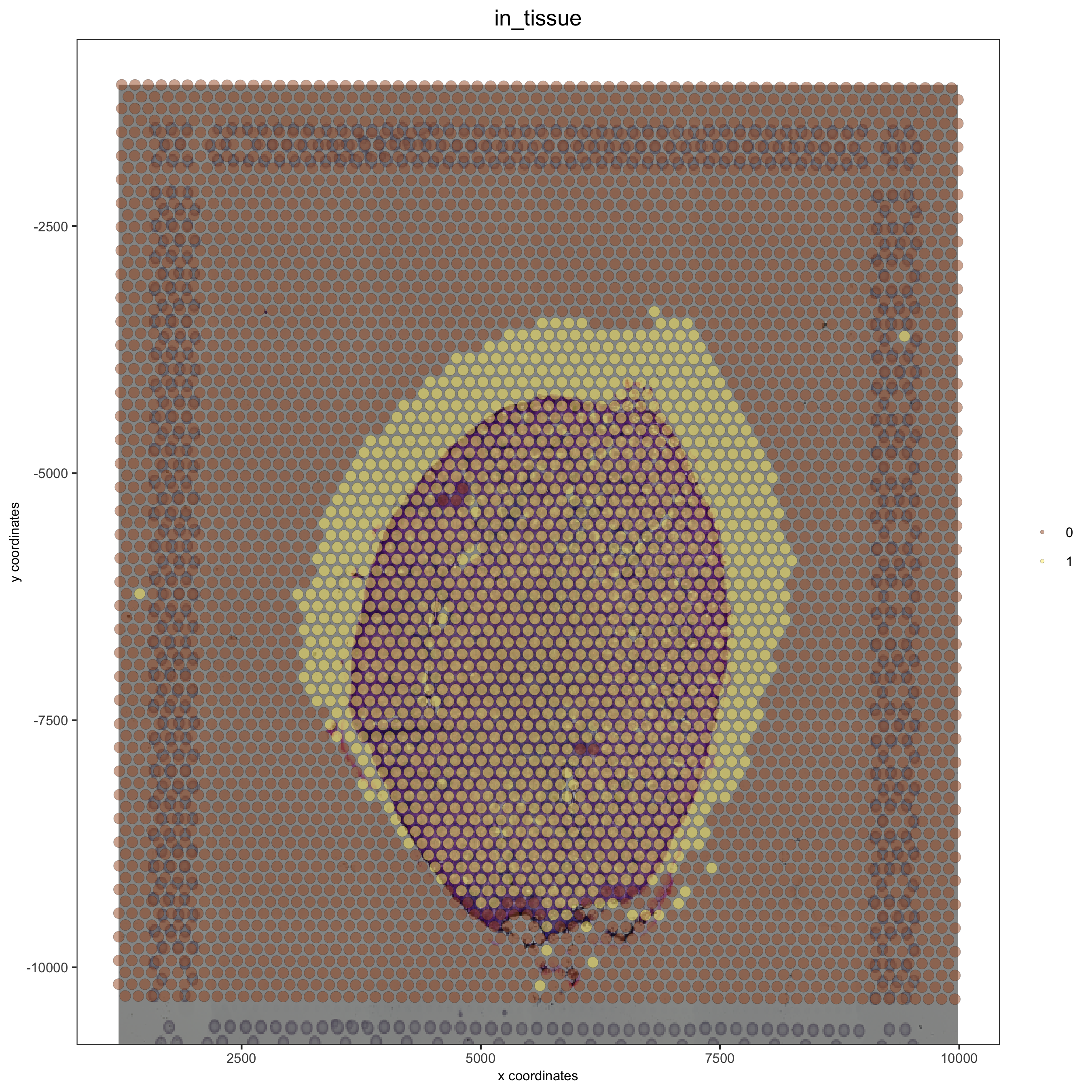
Left Adjustment <– with xmin_adj:
## adjust to left side with xmin_adj
visium_kidney = updateGiottoImage(visium_kidney, image_name = 'image',
                  xmax_adj = 0, xmin_adj = 1000,
                  ymax_adj = 0, ymin_adj = 0)

spatPlot(gobject = visium_kidney, cell_color = 'in_tissue', show_image = T, point_alpha = 0.5)
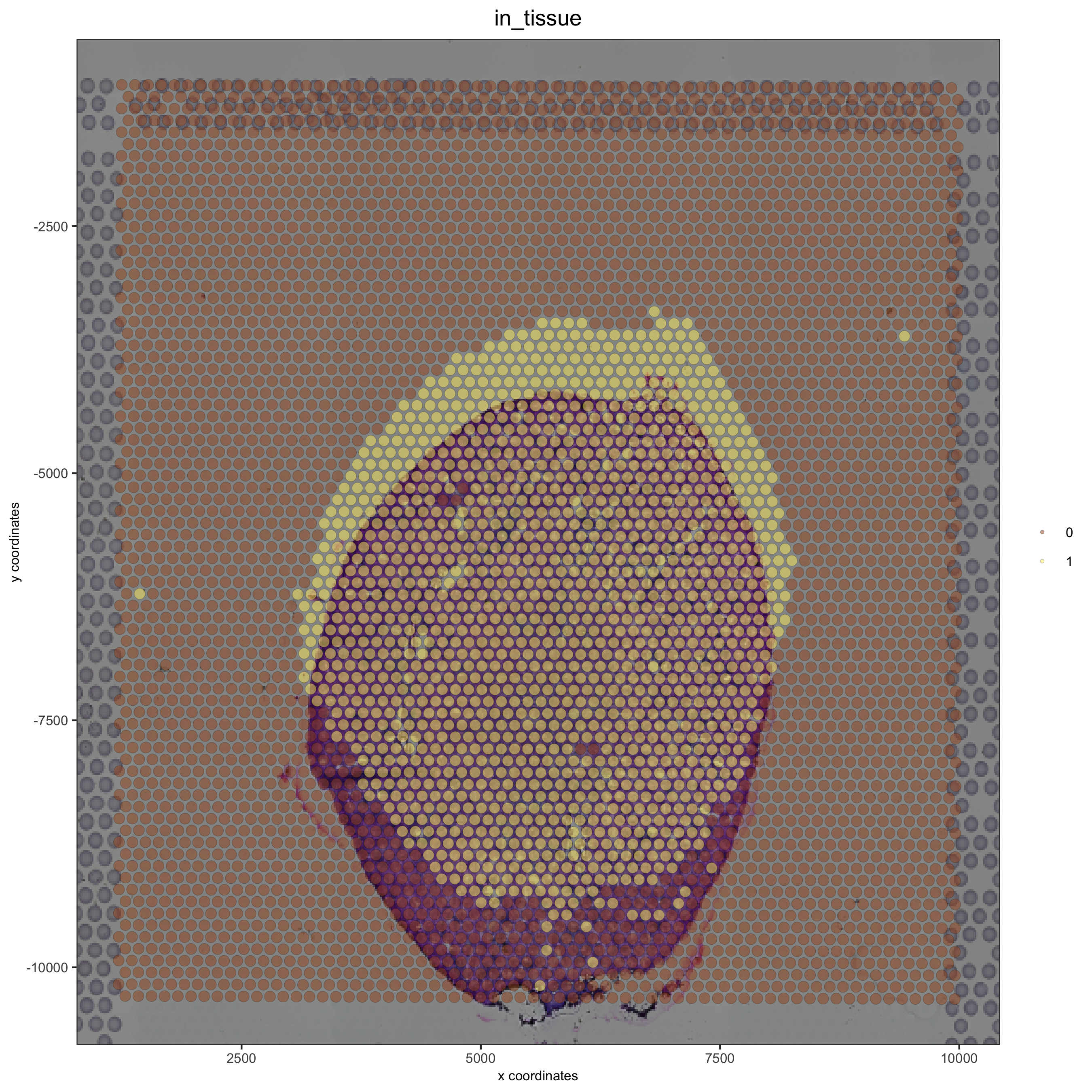
Adjustment to the Top with ymax_adj:
## adjust to top side with ymax_adj
visium_kidney = updateGiottoImage(visium_kidney, image_name = 'image',
              xmax_adj = 0, xmin_adj = 0,
              ymax_adj = 1000, ymin_adj = 0)

spatPlot(gobject = visium_kidney, cell_color = 'in_tissue', show_image = T, point_alpha = 0.5)
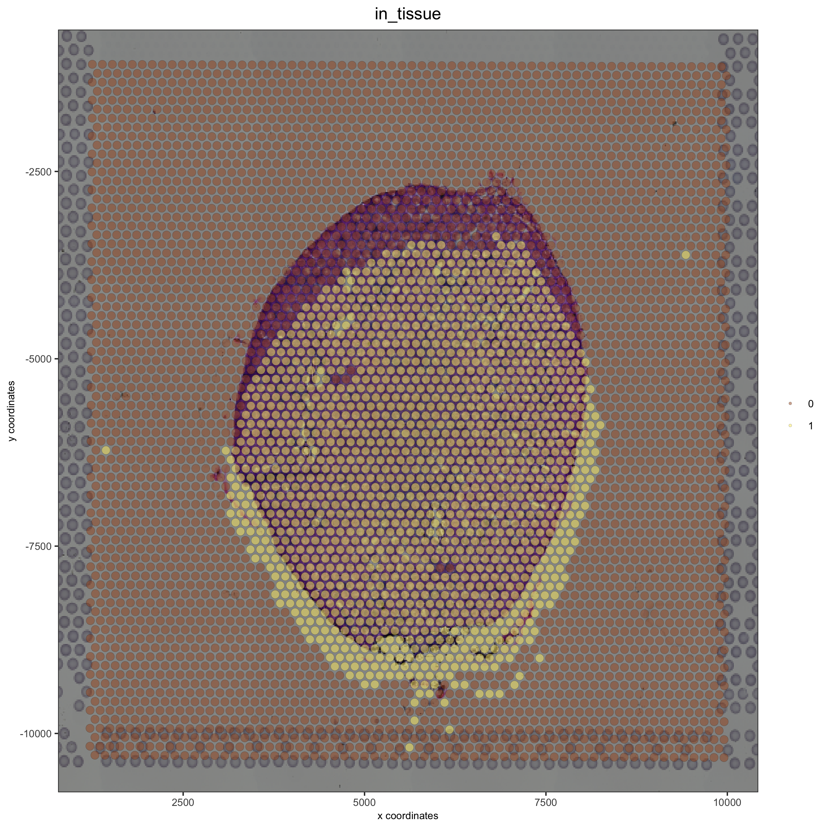
Adjustment to the bottom with ymin_adj:
## adjust to bottom side with ymin_adj
visium_kidney = updateGiottoImage(visium_kidney, image_name = 'image',
              xmax_adj = 0, xmin_adj = 0,
              ymax_adj = 0, ymin_adj = 1000)

spatPlot(gobject = visium_kidney, cell_color = 'in_tissue', show_image = T, point_alpha = 0.5)
Simulation of shifts
Create an OK adjustment:
## OK alignment
visium_kidney = updateGiottoImage(visium_kidney, image_name = 'image',
              xmax_adj = 1000, xmin_adj = 1000,
              ymax_adj = 1000, ymin_adj = 1000)

patPlot(gobject = visium_kidney, cell_color = 'in_tissue', show_image = T, point_alpha = 0.5)
Simulate a right shift and compare with the OK adjustment:
## simulate a right shift
visium_kidney = updateGiottoImage(visium_kidney, image_name = 'image',
              xmax_adj = 2000, xmin_adj = 500,
              ymax_adj = 1000, ymin_adj = 1000)

spatPlot(gobject = visium_kidney, cell_color = 'in_tissue', show_image = T, point_alpha = 0.5)
Simulate a left shift and compare with the OK adjustment:
Simulate a downward shift and compare with the OK adjustment:
## simulate a downward shift
visium_kidney = updateGiottoImage(visium_kidney, image_name = 'image',
              xmax_adj = 1000, xmin_adj = 1000,
              ymax_adj = 500, ymin_adj = 2000)

spatPlot(gobject = visium_kidney, cell_color = 'in_tissue', show_image = T, point_alpha = 0.5)
Simulate a upward shift and compare with the OK adjustment:
## simulate a upward shift
visium_kidney = updateGiottoImage(visium_kidney, image_name = 'image',
              xmax_adj = 1000, xmin_adj = 1000,
              ymax_adj = 2000, ymin_adj = 500)

spatPlot(gobject = visium_kidney, cell_color = 'in_tissue', show_image = T, point_alpha = 0.5)
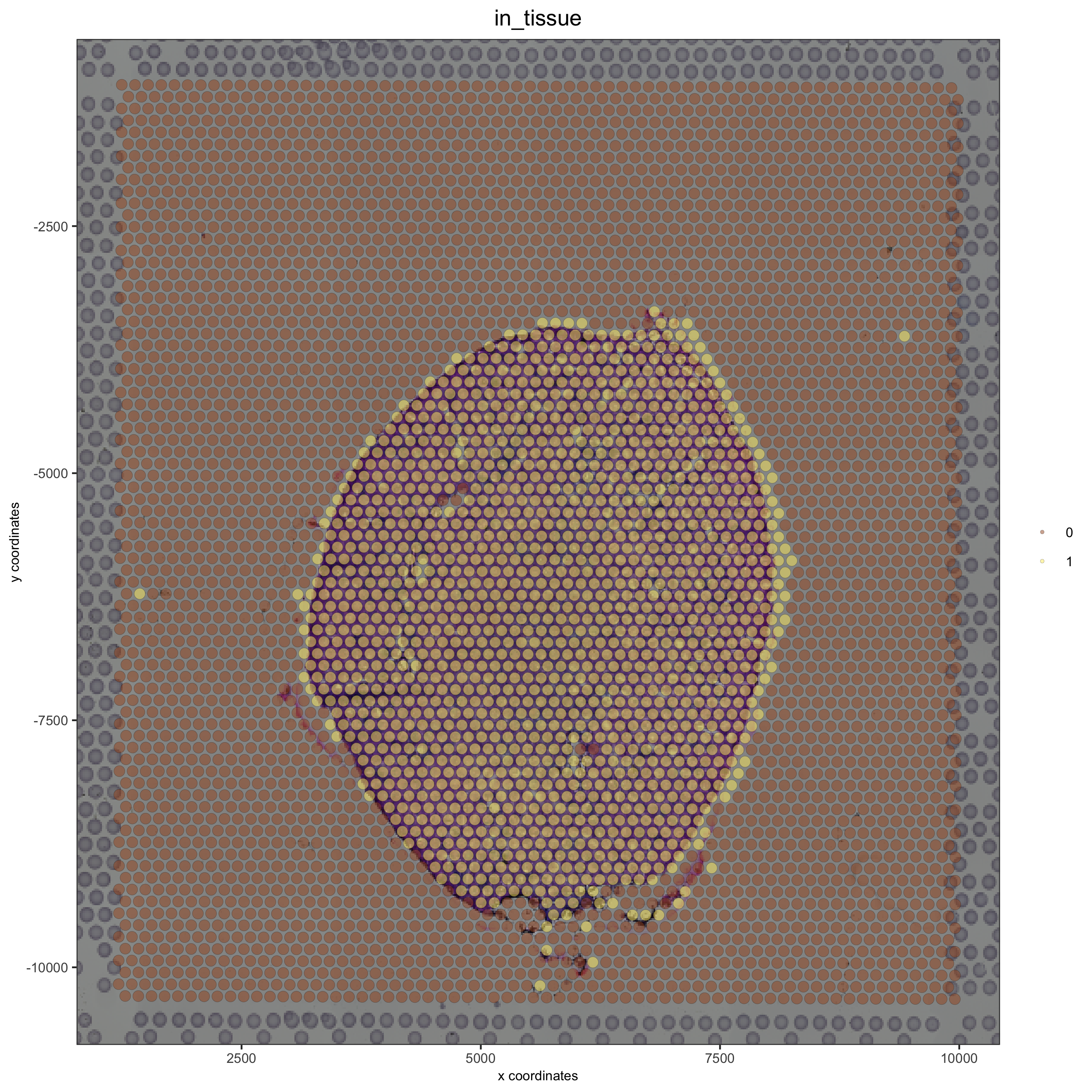
A Good Alignment
# check name
showGiottoImageNames(visium_kidney)
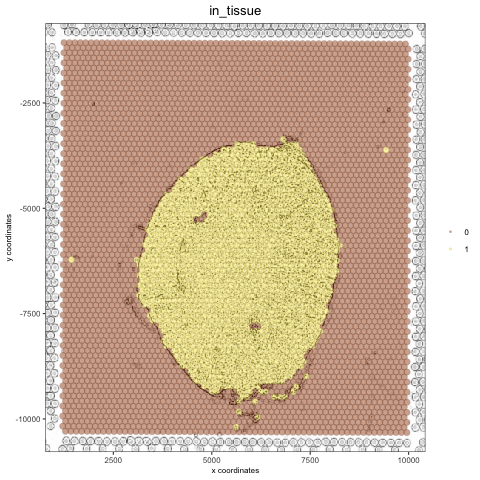
visium_kidney = updateGiottoImage(visium_kidney, image_name = 'image',
xmax_adj = 1300, xmin_adj = 1200,
ymax_adj = 1100, ymin_adj = 1000)
spatPlot(gobject = visium_kidney, cell_color = 'in_tissue', show_image = T, point_alpha = 0.7)
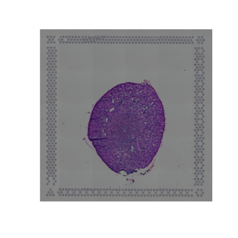
# plot original image
plotGiottoImage(visium_kidney, 'image')
3. Change Background of a Giotto or Magick Image
Extract the giotto image from your giotto object and then estimate the background of your image:
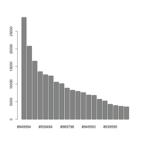
myimage = getGiottoImage(visium_kidney, image_name = 'image') # extract image to modify
estimateImageBg(mg_object = myimage, top_color_range = 1:20)  # estimate background (bg) color
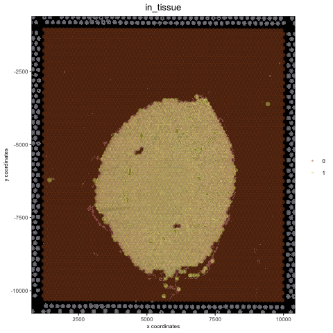
## create and test black background
orig_black_png = changeImageBg(mg_object = myimage, bg_color = '#949594', perc_range = 10, new_color = '#000000', new_name = 'black_bg')

mypl = spatPlot(gobject = visium_kidney, cell_color = 'in_tissue', return_plot = T, point_alpha = 0.5)
mypl_image = addGiottoImageToSpatPlot(mypl, orig_black_png)
mypl_image
## create and test white background
orig_white_png = changeImageBg(mg_object = myimage, bg_color = '#949594', perc_range = 10, new_color = '#FFFFFF', new_name = 'white_bg')

mypl = spatPlot(gobject = visium_kidney, cell_color = 'in_tissue', return_plot = T, point_alpha = 0.5)
mypl_image = addGiottoImageToSpatPlot(mypl, orig_white_png)
mypl_image
4. Add Image From Scratch
## use magick library to load (and optionally modify) figure ##
# original image
png_path = '/your/data/path/Visium_data/Kidney_data/spatial/tissue_lowres_image.png'
mg_img = magick::image_read(png_path)
Create a negated image
# original image negated
mg_img2 = magick::image_negate(mg_img)
orig_neg_png = createGiottoImage(gobject = visium_kidney, mg_object = mg_img2, name = 'image_neg',
             xmax_adj = 1300, xmin_adj = 1200, ymax_adj = 1100, ymin_adj = 1000)
mypl_image = addGiottoImageToSpatPlot(mypl, orig_neg_png)
mypl_image

Create a charcoal image
# charcoal image (black/white)
mg_img3 = magick::image_charcoal(mg_img, radius = 1)
mg_img3 = magick::image_convert(mg_img3, colorspace = 'rgb')
orig_charc_png = createGiottoImage(gobject = visium_kidney, mg_object = mg_img3, name = 'image_charc',
               xmax_adj = 1300, xmin_adj = 1200, ymax_adj = 1100, ymin_adj = 1000)
mypl_image = addGiottoImageToSpatPlot(mypl, orig_charc_png)
mypl_image
Add multiple new images to your giotto object
## add images to Giotto object ##
image_list = list(orig_white_png, orig_black_png, orig_neg_png, orig_charc_png)
visium_kidney = addGiottoImage(gobject = visium_kidney,
               images = image_list)
showGiottoImageNames(visium_kidney) # shows which Giotto images are attached to you Giotto object
5. Example: Kidney Analysis
5.1 Processing
## subset on spots that were covered by tissue
metadata = pDataDT(visium_kidney)
in_tissue_barcodes = metadata[in_tissue == 1]$cell_ID
visium_kidney = subsetGiotto(visium_kidney, cell_ids = in_tissue_barcodes)
## filter
visium_kidney <- filterGiotto(gobject = visium_kidney,
expression_threshold = 1,
gene_det_in_min_cells = 50,
min_det_genes_per_cell = 1000,
expression_values = c('raw'),
verbose = T)
## normalize
visium_kidney <- normalizeGiotto(gobject = visium_kidney, scalefactor = 6000, verbose = T)
## add gene & cell statistics
visium_kidney <- addStatistics(gobject = visium_kidney)
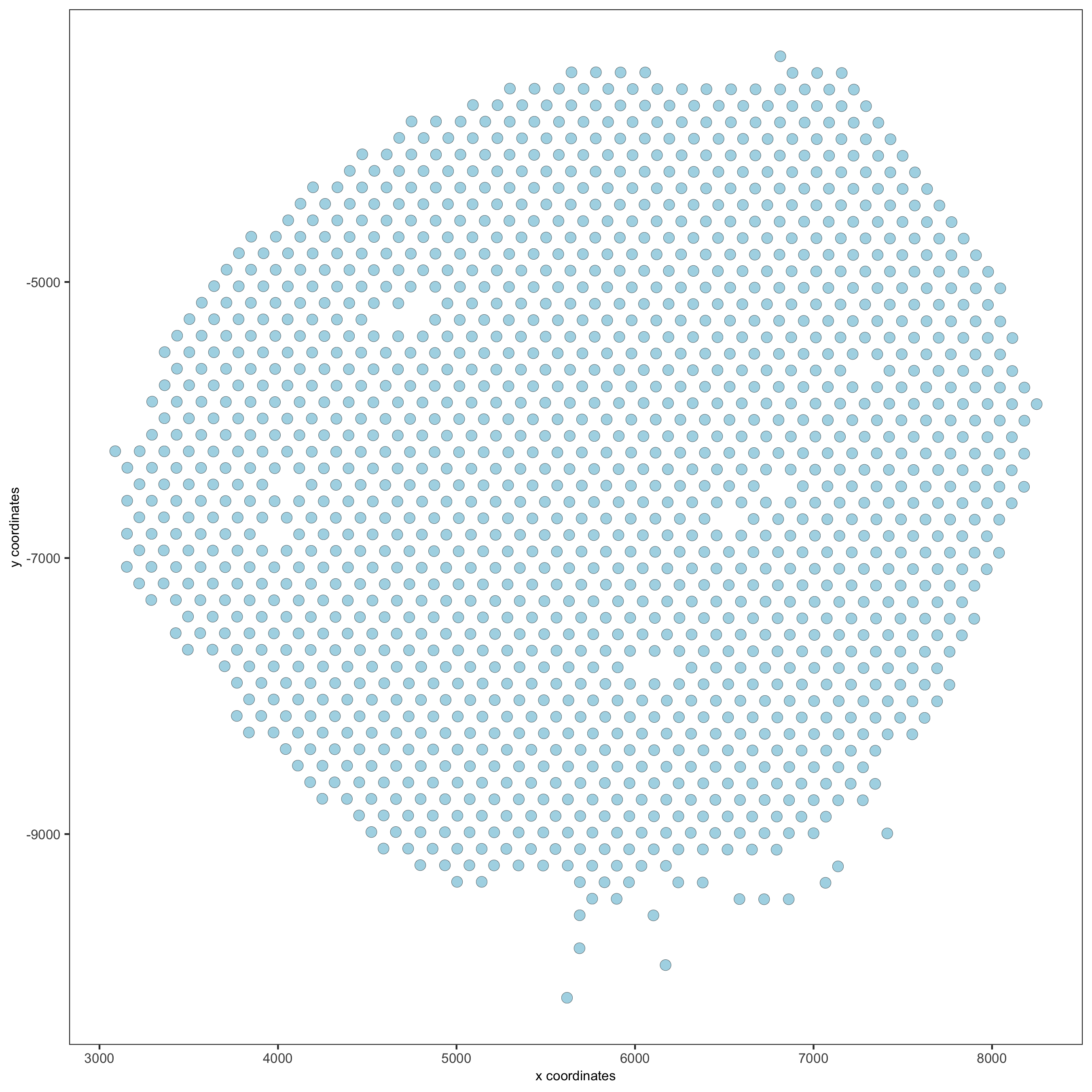
## visualize
spatPlot(gobject = visium_kidney)
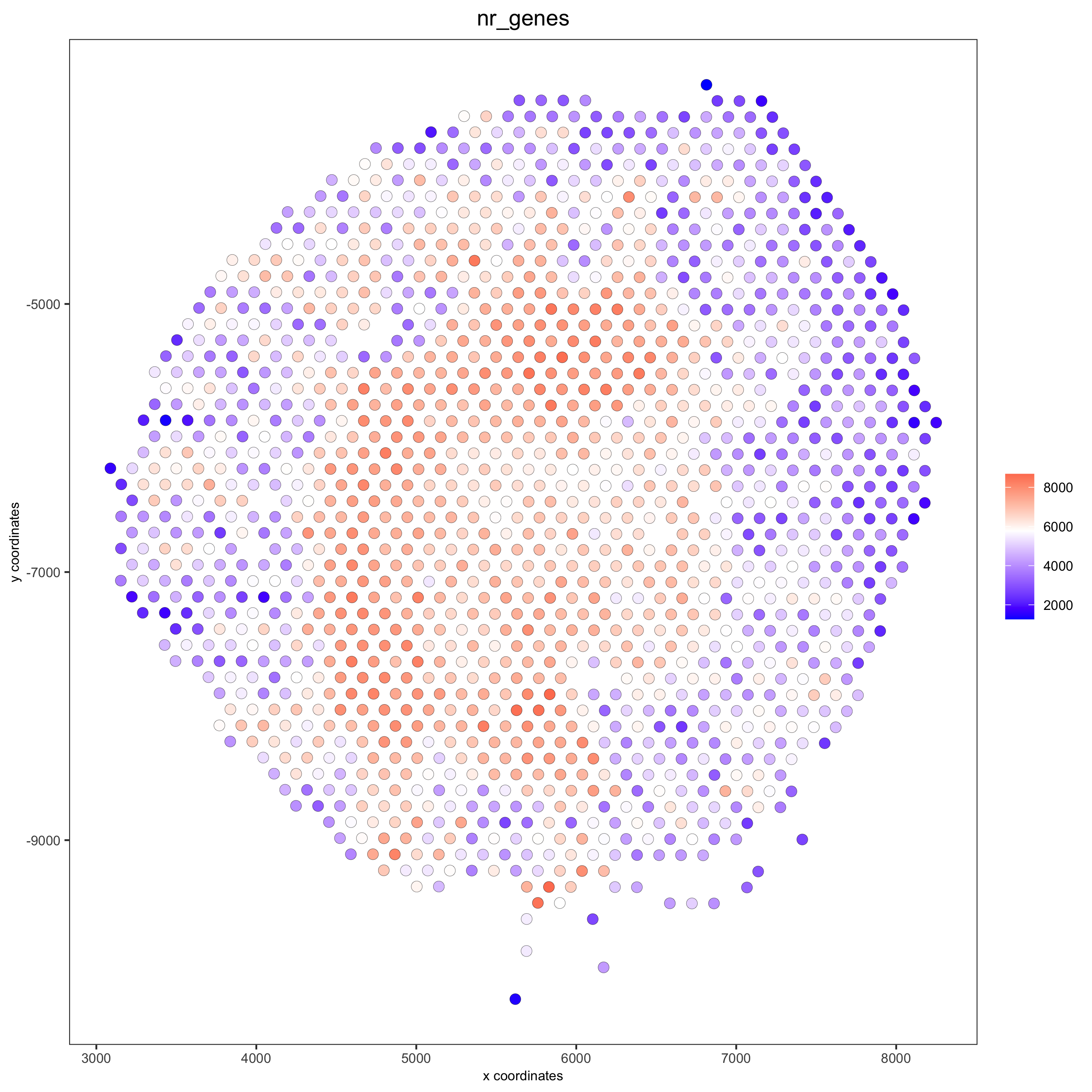
spatPlot(gobject = visium_kidney, cell_color = 'nr_genes', color_as_factor = F)
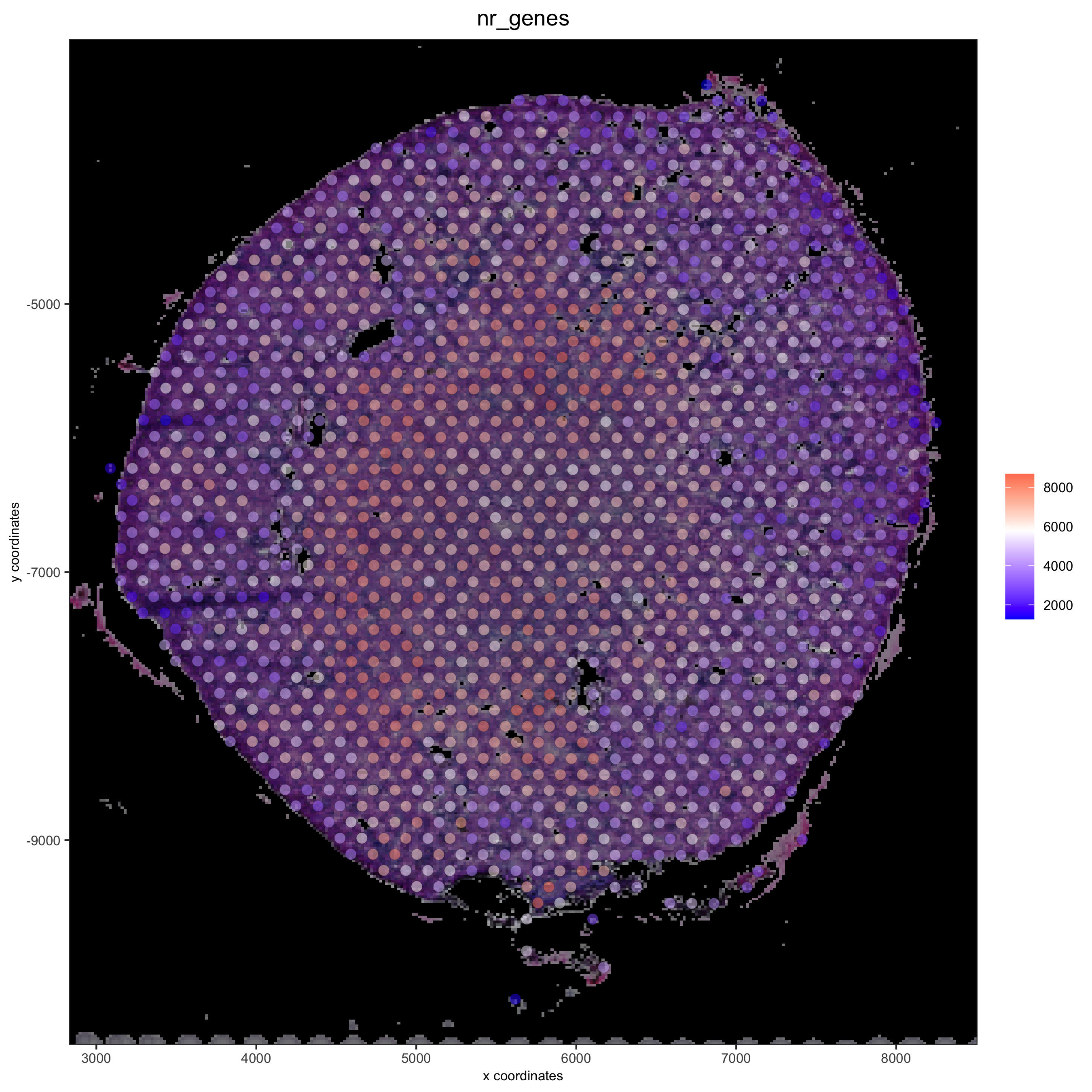
# add black background image
spatPlot(gobject = visium_kidney, show_image = T, image_name = "black_bg",
    cell_color = 'nr_genes', color_as_factor = F, point_alpha = 0.5)
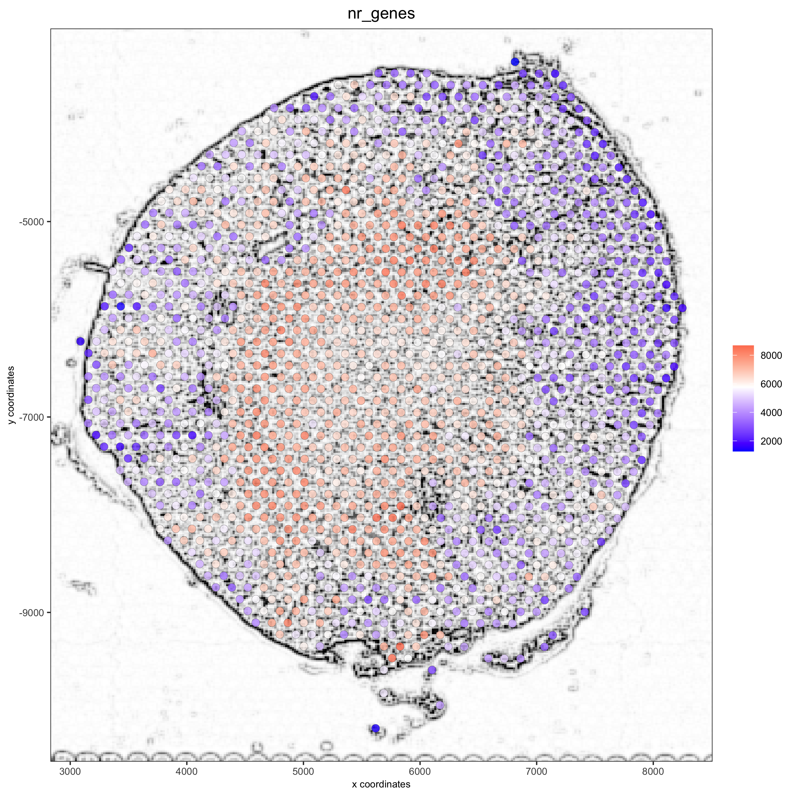
## alternative: directly provide a gimage (giotto image object), this will override the the image_name param
spatPlot(gobject = visium_kidney, show_image = T, gimage = orig_charc_png,
    cell_color = 'nr_genes', color_as_factor = F, point_alpha = 0.8)
5.2 Dimension Reduction
## highly variable genes (HVG)
visium_kidney <- calculateHVG(gobject = visium_kidney, nr_expression_groups = 10)
## select genes based on HVG and gene statistics, both found in gene metadata
gene_metadata = fDataDT(visium_kidney)
featgenes = gene_metadata[hvg == 'yes' & perc_cells > 4 & mean_expr_det > 0.5]$gene_ID
## run PCA on expression values (default)
visium_kidney <- runPCA(gobject = visium_kidney, genes_to_use = featgenes)
## run UMAP and tSNE on PCA space (default)
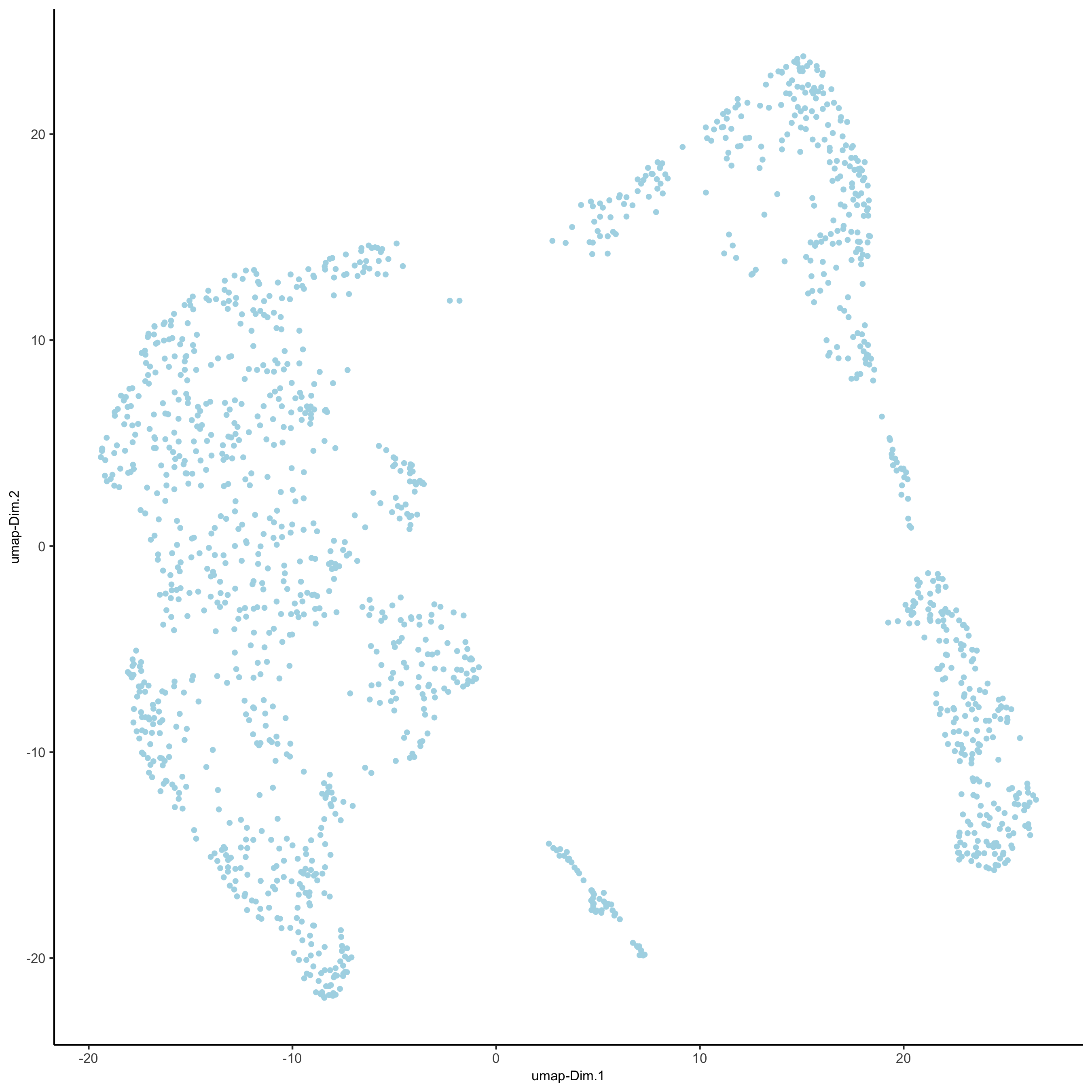
visium_kidney <- runUMAP(visium_kidney, dimensions_to_use = 1:10)
plotUMAP(gobject = visium_kidney)
5.3 Cluster
## sNN network (default)
visium_kidney <- createNearestNetwork(gobject = visium_kidney, dimensions_to_use = 1:10, k = 15)
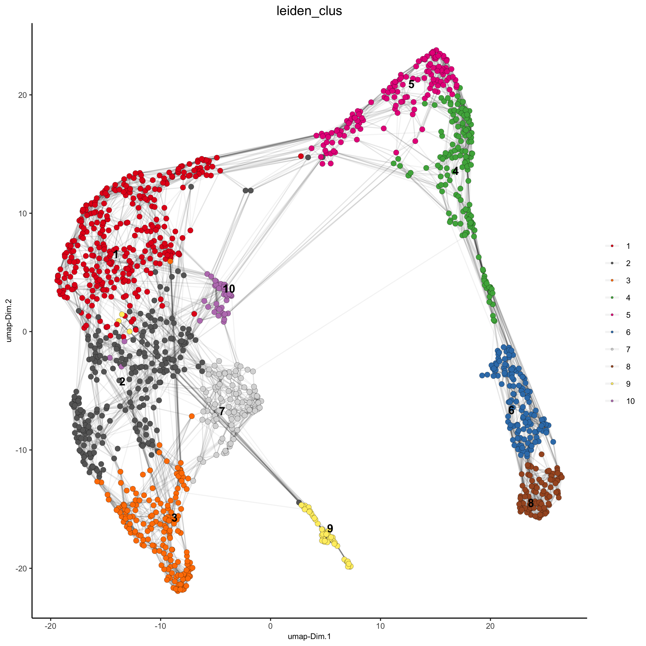
## Leiden clustering
visium_kidney <- doLeidenCluster(gobject = visium_kidney, resolution = 0.4, n_iterations = 1000)
plotUMAP(gobject = visium_kidney,
cell_color = 'leiden_clus', show_NN_network = T, point_size = 2.5)
5.4 Co-Visualize
# expression and spatial
showGiottoImageNames(visium_kidney)
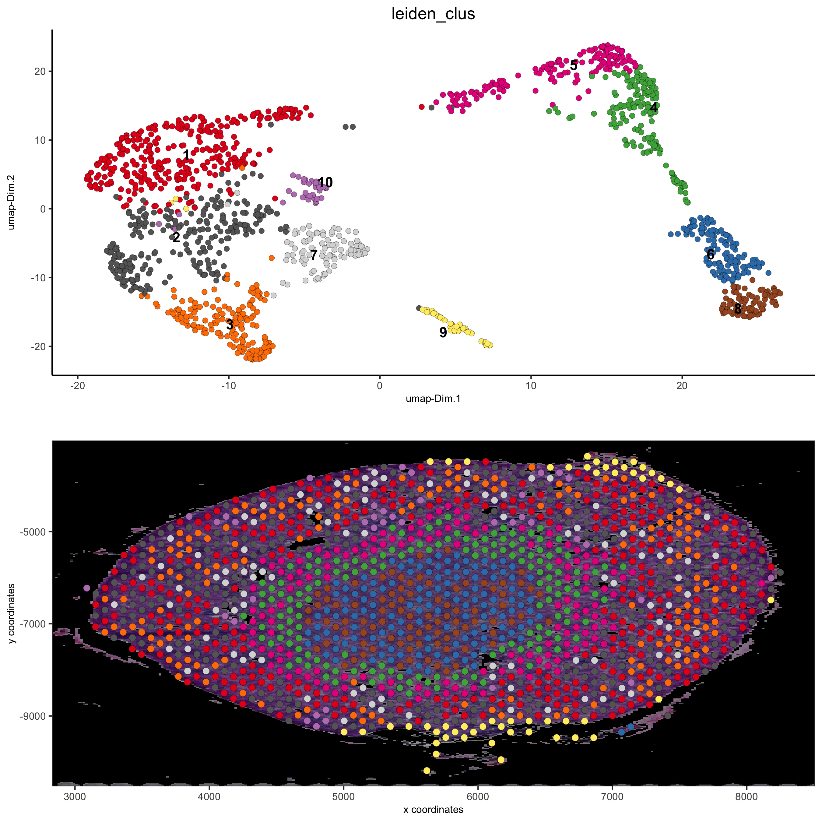
spatDimPlot(gobject = visium_kidney, cell_color = 'leiden_clus',
show_image = T, image_name = 'black_bg',
dim_point_size = 2, spat_point_size = 2.5,
save_param = list(save_name = '7_a_covis_leiden_black'))
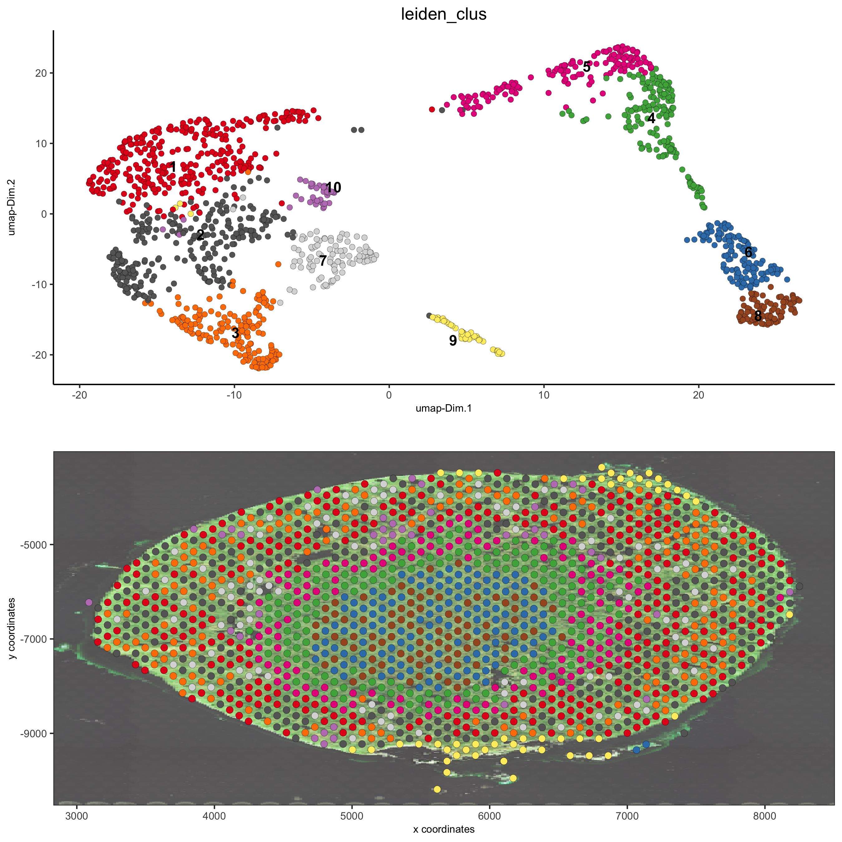
spatDimPlot(gobject = visium_kidney, cell_color = 'leiden_clus',
    show_image = T, image_name = 'image_neg',
    dim_point_size = 2, spat_point_size = 2.5,
    save_param = list(save_name = '7_b_covis_leiden_negated'))
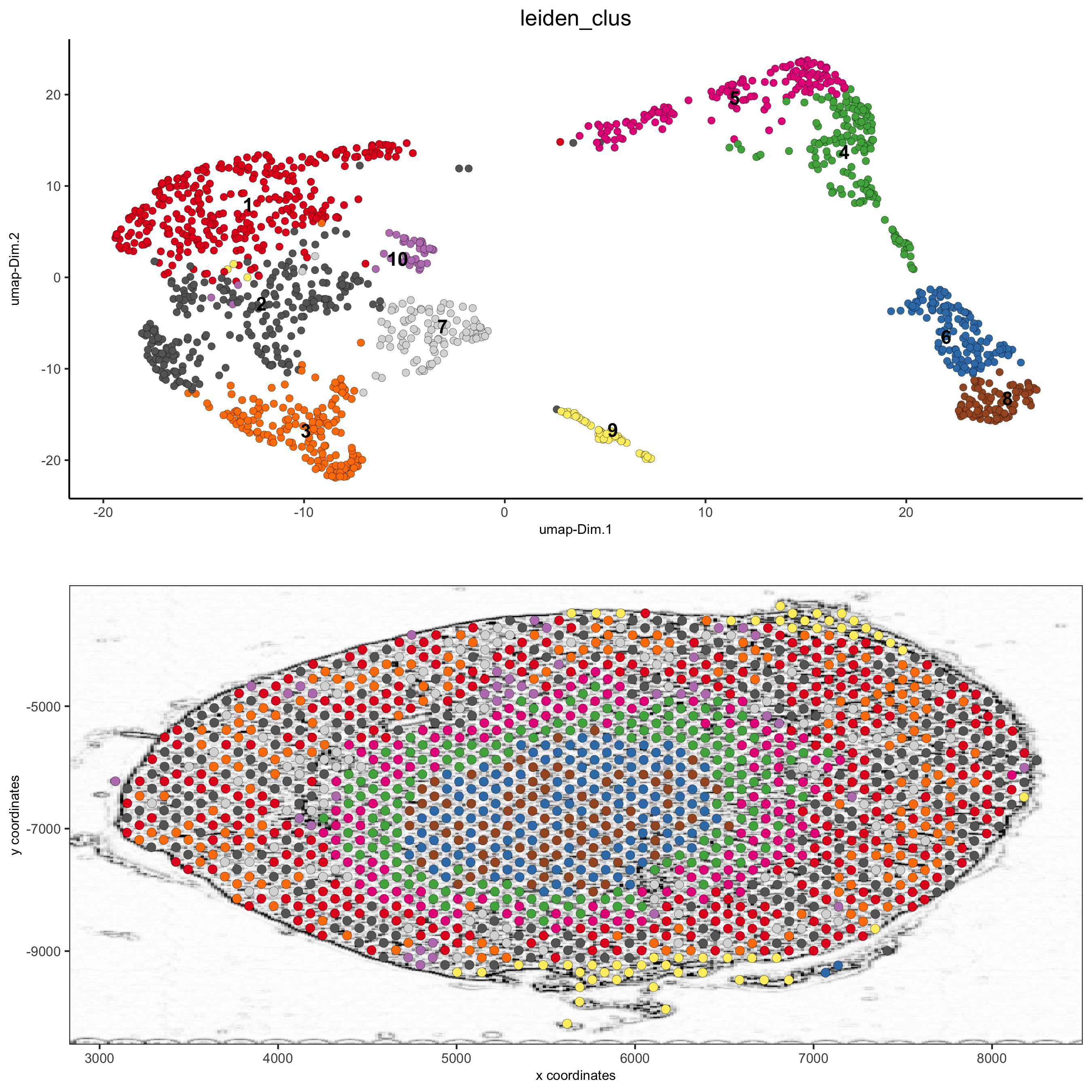
spatDimPlot(gobject = visium_kidney, cell_color = 'leiden_clus',
    show_image = T, image_name = 'image_charc',
    dim_point_size = 2, spat_point_size = 2.5,
    save_param = list(save_name = '7_b_covis_leiden_charc'))
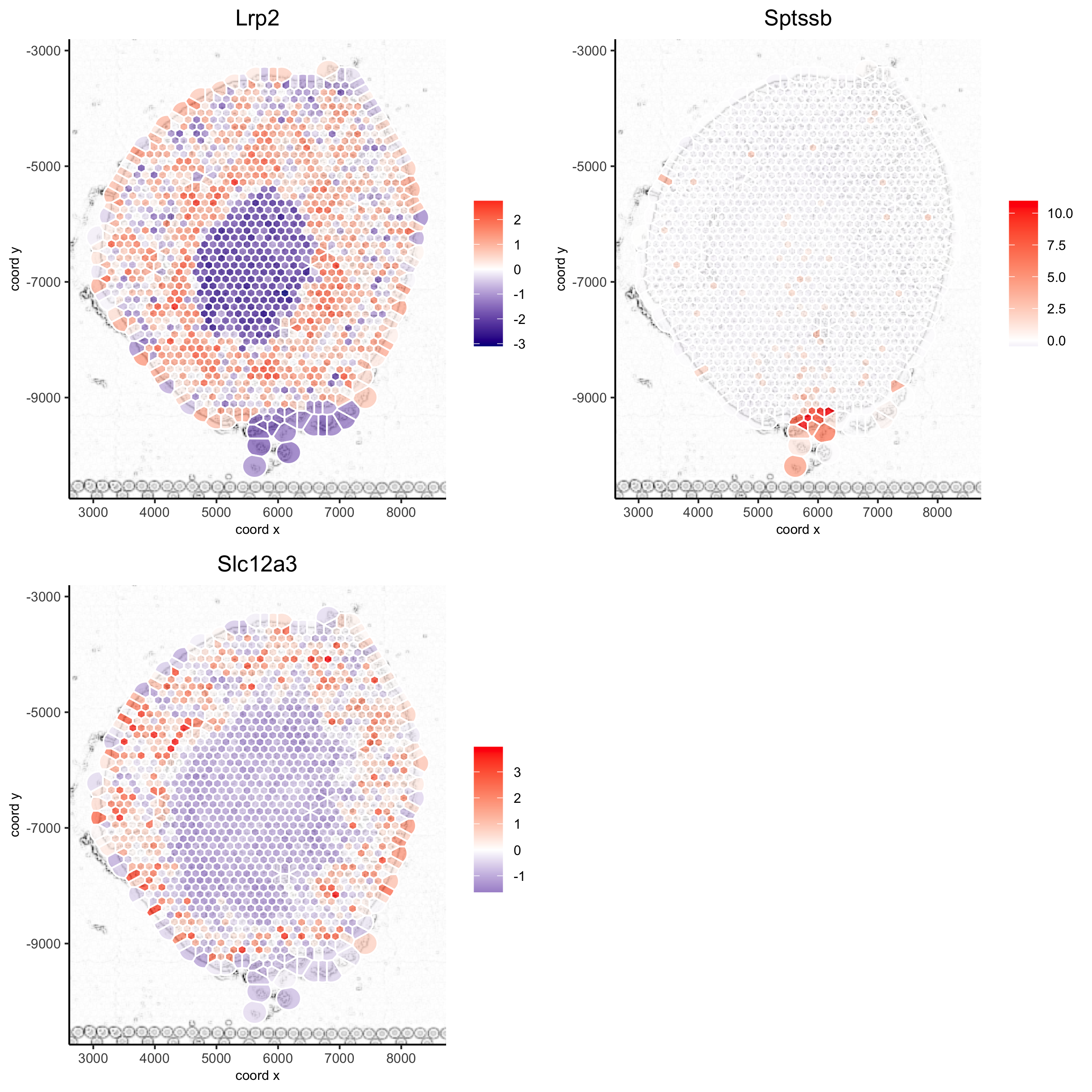
5.5 Spatial Gene Plots
## gene plots ##
spatGenePlot(visium_kidney, show_image = T, image_name = 'image_charc',
    expression_values = 'scaled', point_size = 2,
    genes = c('Lrp2', 'Sptssb', 'Slc12a3'),  cow_n_col = 2,
    cell_color_gradient = c('darkblue', 'white', 'red'), gradient_midpoint = 0, point_alpha = 0.8,
    save_param = list(save_name = '8_a_spatgene_charc'))
spatGenePlot(visium_kidney, show_image = T, image_name = 'image_charc',
    expression_values = 'scaled', point_size = 2, point_shape = 'voronoi',
    genes = c('Lrp2', 'Sptssb', 'Slc12a3'),  cow_n_col = 2,
    cell_color_gradient = c('darkblue', 'white', 'red'), gradient_midpoint = 0, vor_alpha = 0.8,
    save_param = list(save_name = '8_b_spatgene_charc_vor'))

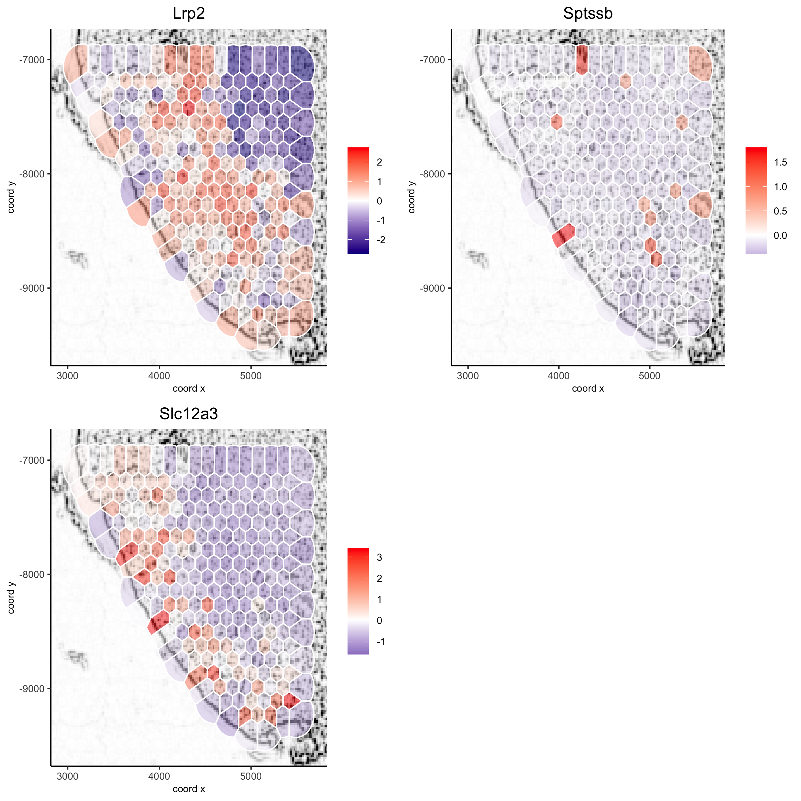
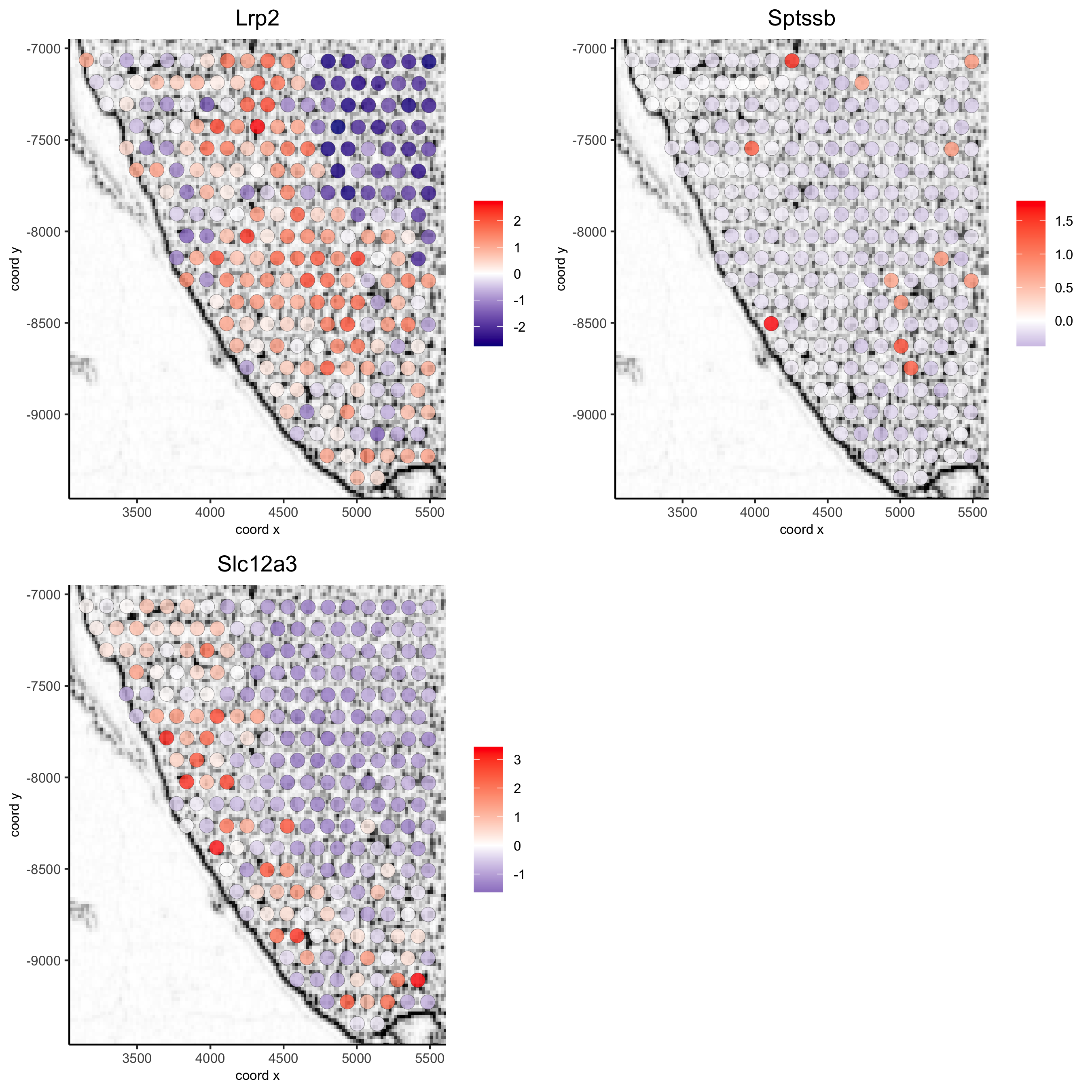
5.6 Subset Plots
visium_kidney_subset = subsetGiottoLocs(visium_kidney, x_min = 3000, x_max = 5500, y_min = -10000, y_max = -7000)

spatGenePlot(visium_kidney_subset, show_image = T, image_name = 'image_charc',
    expression_values = 'scaled', point_size = 4,
    genes = c('Lrp2', 'Sptssb', 'Slc12a3'),  cow_n_col = 2,
    cell_color_gradient = c('darkblue', 'white', 'red'), gradient_midpoint = 0,
    point_alpha = 0.8,
    save_param = list(save_name = '9_a_subset_spatgene_charc'))
spatGenePlot(visium_kidney_subset, show_image = T, image_name = 'image_charc',
    expression_values = 'scaled', point_size = 4,  point_shape = 'voronoi', vor_alpha = 0.5,
    genes = c('Lrp2', 'Sptssb', 'Slc12a3'),  cow_n_col = 2,
    cell_color_gradient = c('darkblue', 'white', 'red'), gradient_midpoint = 0,
    save_param = list(save_name = '9_b_subset_spatgene_charc_vor'))