Mouse Visium Kidney

Warning

This tutorial was written with Giotto version 0.3.6.9046, your version is 1.0.3. This is a more recent version and results should be reproducible.

Install Python and R Modules

To run this vignette you need to install all of the necessary Python modules.

Important

Python module installation can be done either automatically via our installation tool (from within R) (see step 2.2A) or manually (see step 2.2B).

See Part 2.2 Giotto-Specific Python Packages of our Giotto Installation section for step-by-step instructions.

Optional: Set Giotto Instructions

Within R

# to automatically save figures in save_dir set save_plot to TRUE
temp_dir = getwd()
temp_dir = '~/Temp/'
myinstructions = createGiottoInstructions(save_dir = temp_dir,
                      save_plot = TRUE,
                      show_plot = FALSE)

Set-Up Giotto

library(Giotto)

Set A Working Directory

#results_folder = '/path/to/directory/'
results_folder = '/Volumes/Ruben_Seagate/Dropbox (Personal)/Projects/GC_lab/Ruben_Dries/190225_spatial_package/Results/Visium/Brain/201226_results//'

Set A Giotto Python Path

# set python path to your preferred python version path
# set python path to NULL if you want to automatically install (only the 1st time) and use the giotto miniconda environment
python_path = NULL
if(is.null(python_path)) {
    installGiottoEnvironment()
}

Dataset Explanation

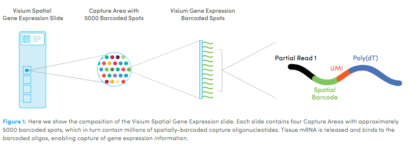
10X genomics recently launched a new platform to obtain spatial expression data using a Visium Spatial Gene Expression slide. The Visium brain data to run this tutorial can be found here.

Important

Visium Technology

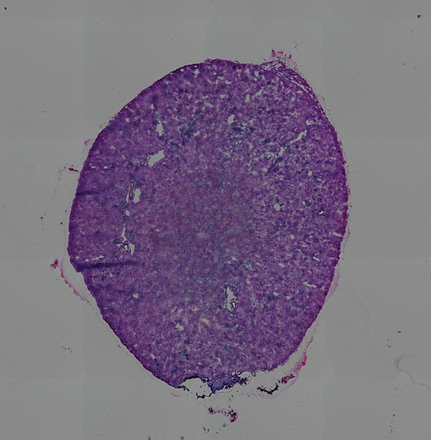
High resolution png from original tissue:

1. Giotto Global Instructions and Preparations

1.1. Create Instructions

instrs = createGiottoInstructions(save_dir = results_folder,
              save_plot = TRUE,
              show_plot = FALSE,
              python_path = python_path)

1.2. Provide Path to Visium Folder

data_path = '/path/to/Kidney_data/'

2. Create Giotto Object and Process The Data

## directly from visium folder
visium_kidney = createGiottoVisiumObject(visium_dir = data_path, expr_data = 'raw',
                 png_name = 'tissue_lowres_image.png',
                 gene_column_index = 2, instructions = instrs)

# check name
showGiottoImageNames(visium_kidney) # "image" is the default name
# adjust parameters to align image (iterative approach)
visium_kidney = updateGiottoImage(visium_kidney, image_name = 'image',
              xmax_adj = 1300, xmin_adj = 1200,
              ymax_adj = 1100, ymin_adj = 1000)

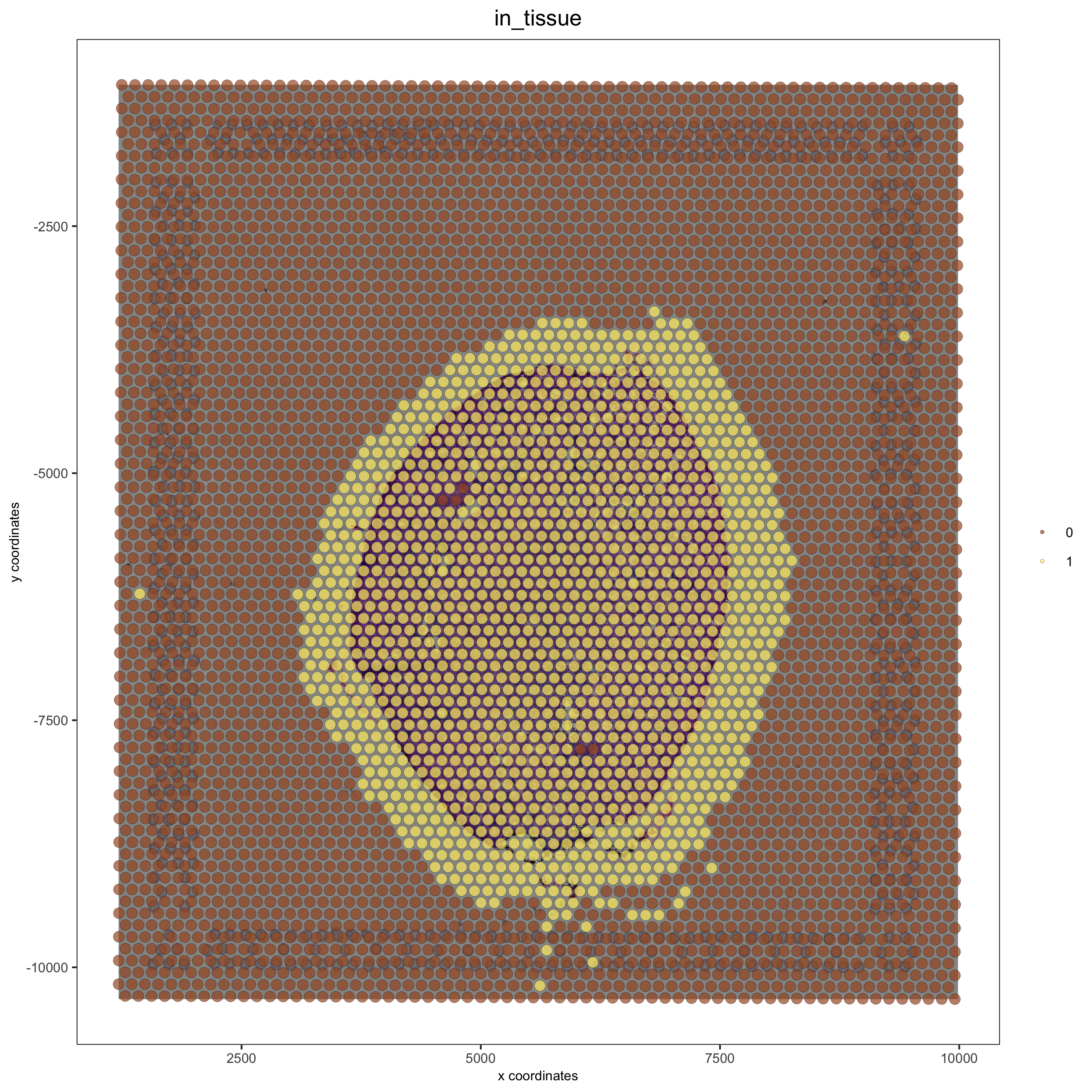
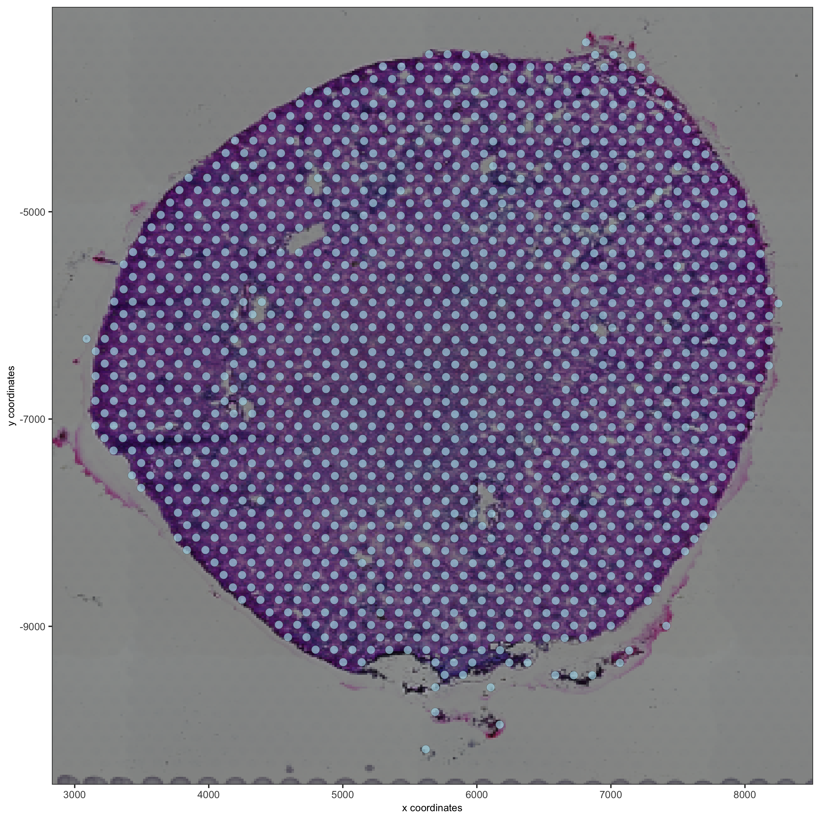
# now it's aligned
spatPlot(gobject = visium_kidney, cell_color = 'in_tissue', show_image = T, point_alpha = 0.7,
    save_param = list(save_name = '2_b_spatplot_image_adjusted'))

## check metadata
pDataDT(visium_kidney)

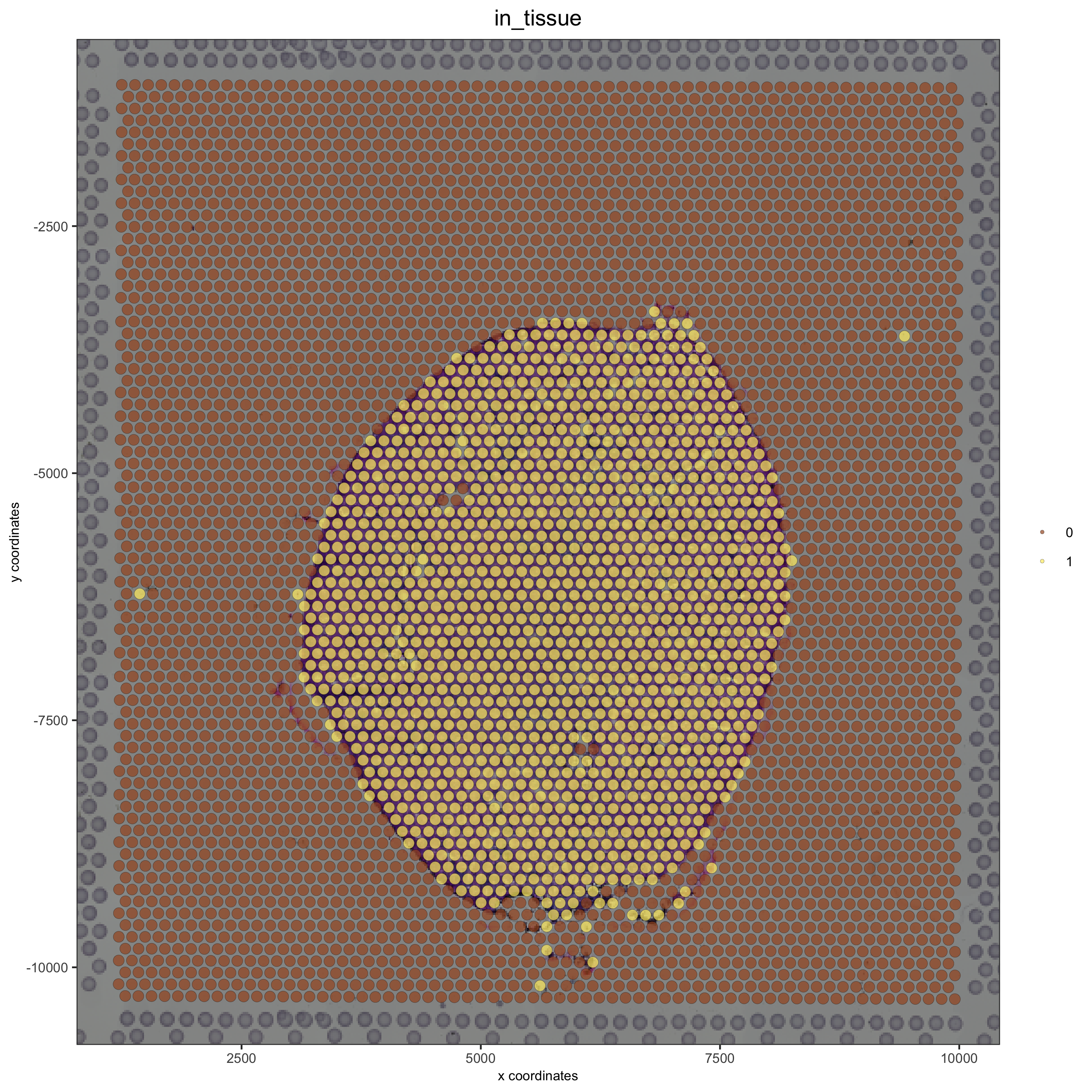
## compare in tissue with provided jpg
spatPlot(gobject = visium_kidney, cell_color = 'in_tissue', point_size = 2,
    cell_color_code = c('0' = 'lightgrey', '1' = 'blue'),
    save_param = list(save_name = '2_c_in_tissue'))

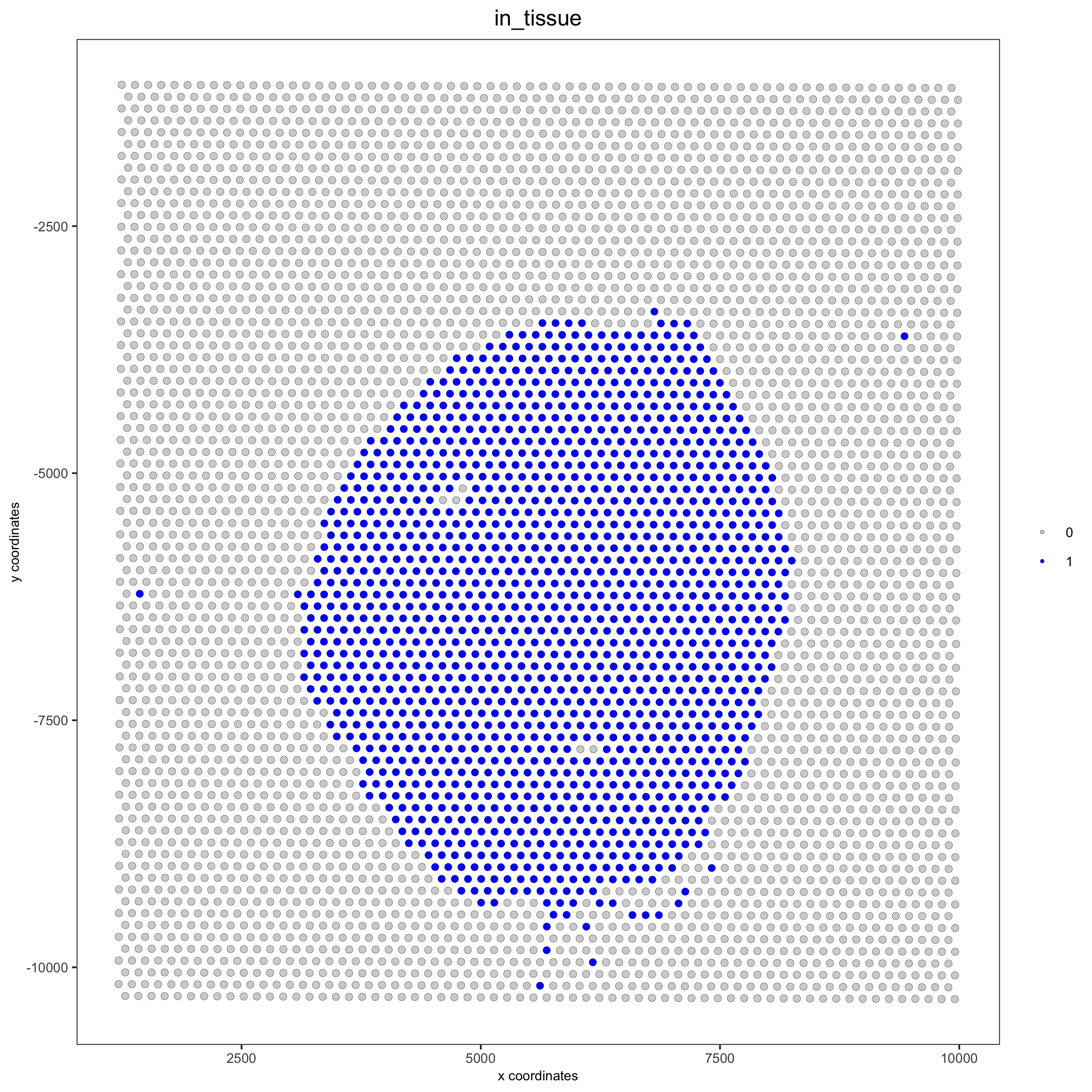
## subset on spots that were covered by tissue
metadata = pDataDT(visium_kidney)
in_tissue_barcodes = metadata[in_tissue == 1]$cell_ID
visium_kidney = subsetGiotto(visium_kidney, cell_ids = in_tissue_barcodes)

## filter
visium_kidney <- filterGiotto(gobject = visium_kidney,
              expression_threshold = 1,
              gene_det_in_min_cells = 50,
              min_det_genes_per_cell = 1000,
              expression_values = c('raw'),
              verbose = T)

## normalize
visium_kidney <- normalizeGiotto(gobject = visium_kidney, scalefactor = 6000, verbose = T)

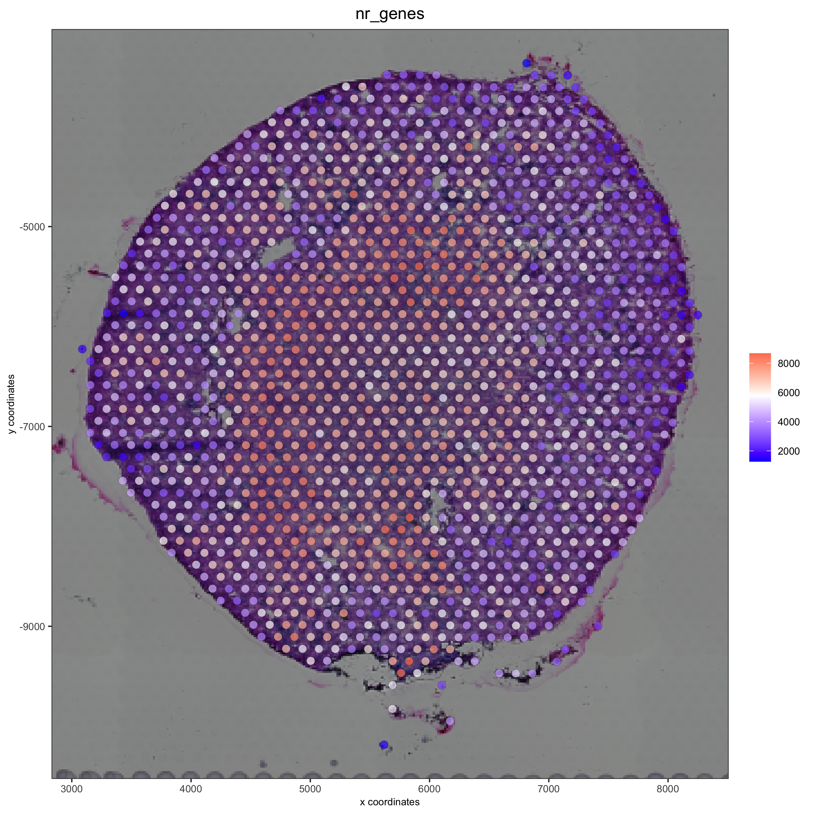
## add gene & cell statistics
visium_kidney <- addStatistics(gobject = visium_kidney)

spatPlot2D(gobject = visium_kidney, show_image = T, point_alpha = 0.7,
   cell_color = 'nr_genes', color_as_factor = F,
   save_param = list(save_name = '2_e_nr_genes'))

3. Dimension Reduction

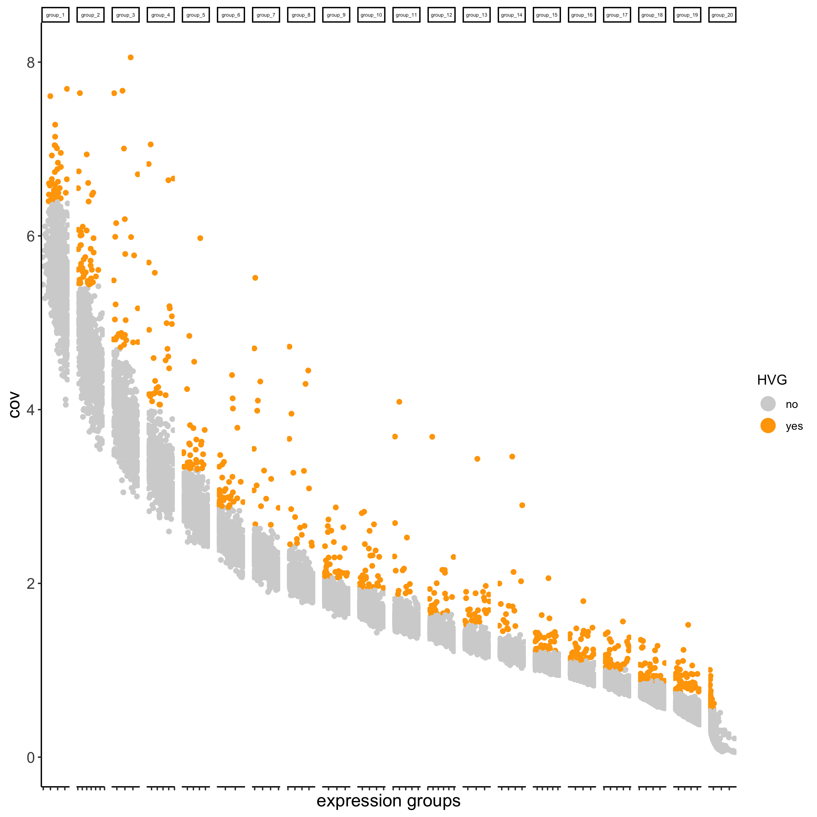
## highly variable genes (HVG)
visium_kidney <- calculateHVG(gobject = visium_kidney,
              save_param = list(save_name = '3_a_HVGplot'))

## run PCA on expression values (default)
visium_kidney <- runPCA(gobject = visium_kidney, center = TRUE, scale_unit = TRUE)
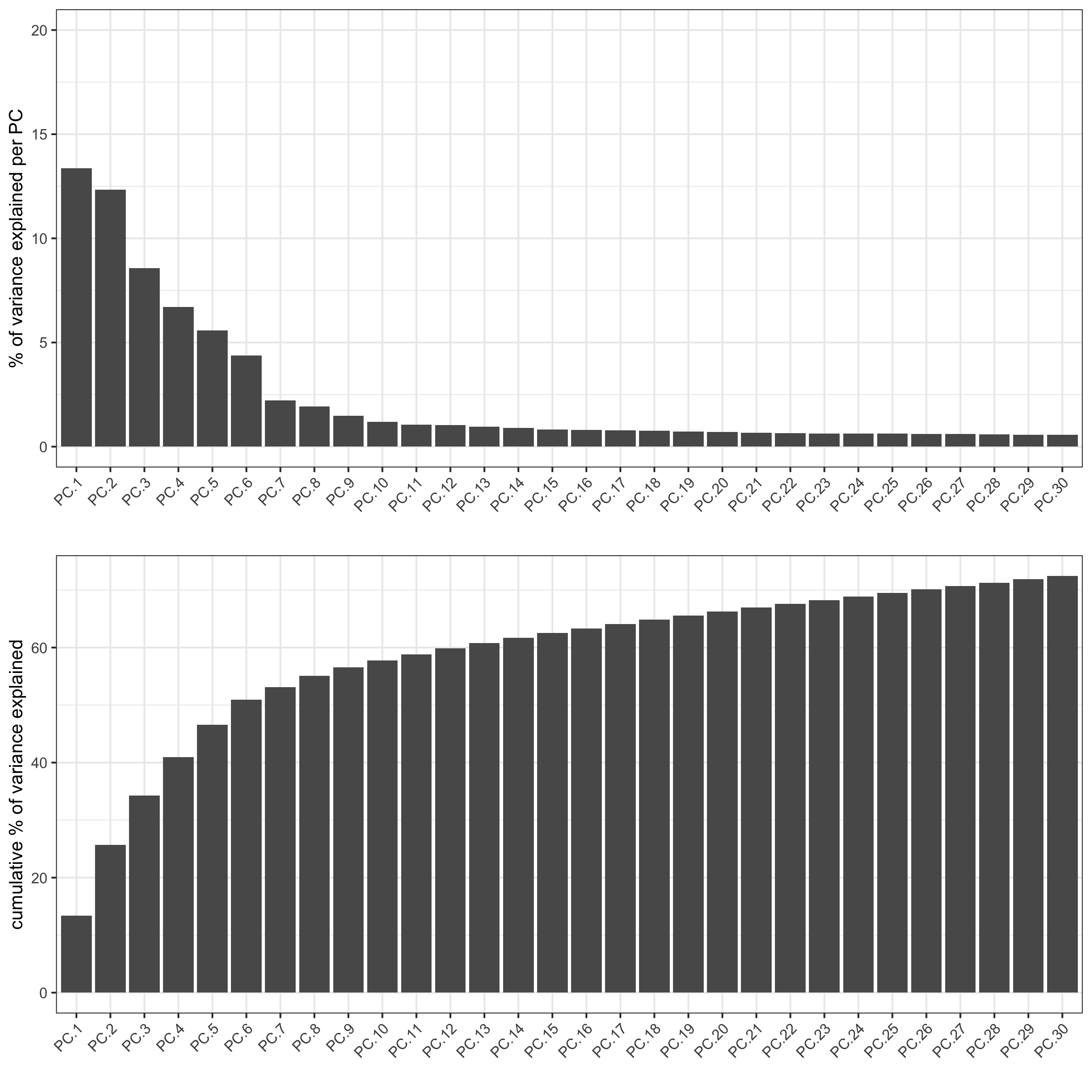
screePlot(visium_kidney, ncp = 30, save_param = list(save_name = '3_b_screeplot'))

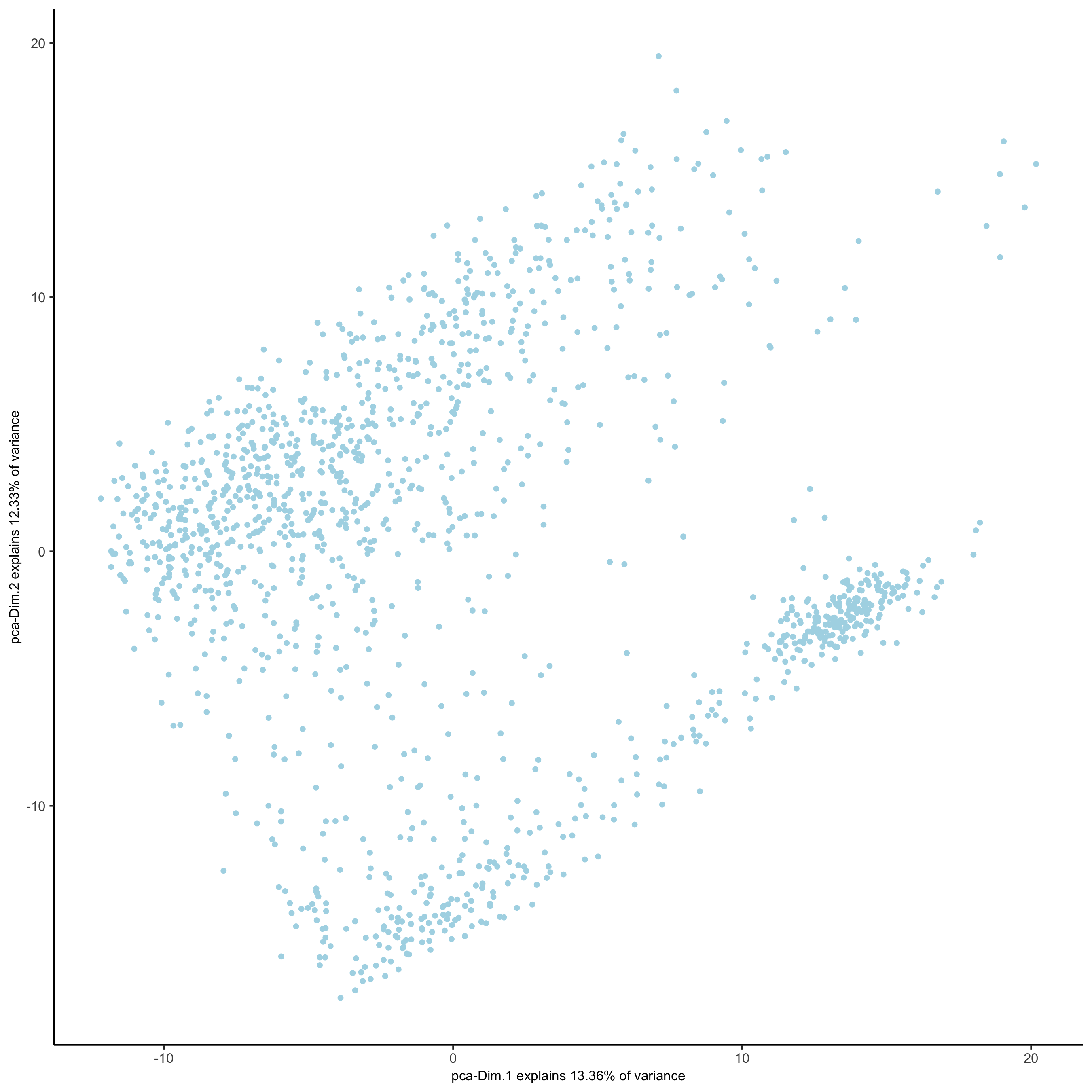
plotPCA(gobject = visium_kidney,
        save_param = list(save_name = '3_c_PCA_reduction'))

## run UMAP and tSNE on PCA space (default)
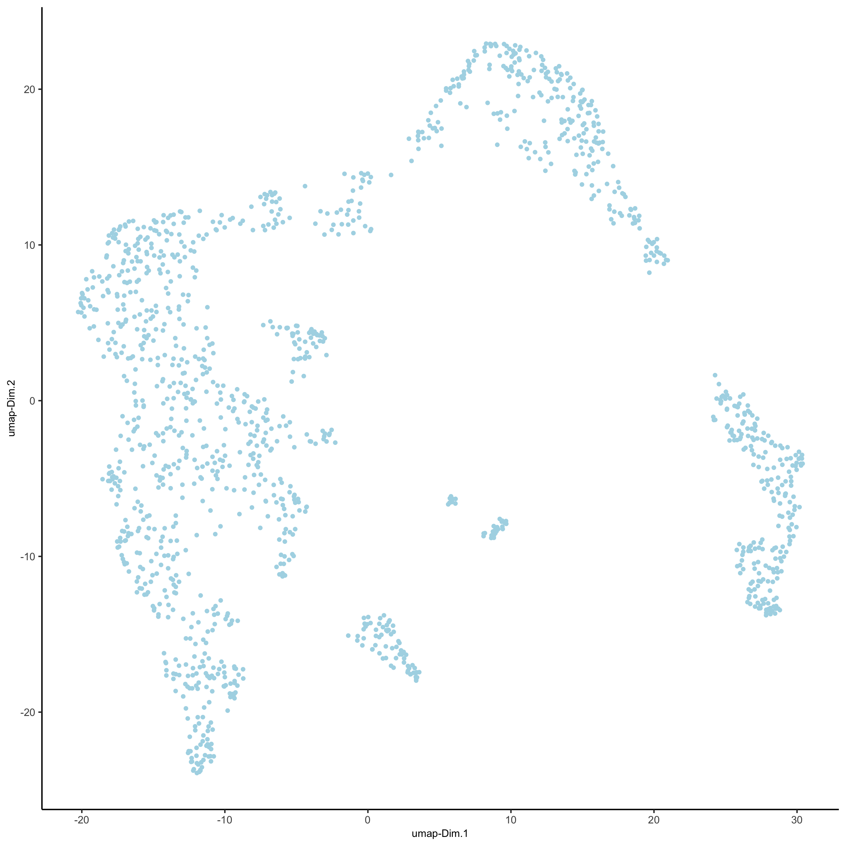
visium_kidney <- runUMAP(visium_kidney, dimensions_to_use = 1:10)
plotUMAP(gobject = visium_kidney,
    save_param = list(save_name = '3_d_UMAP_reduction'))

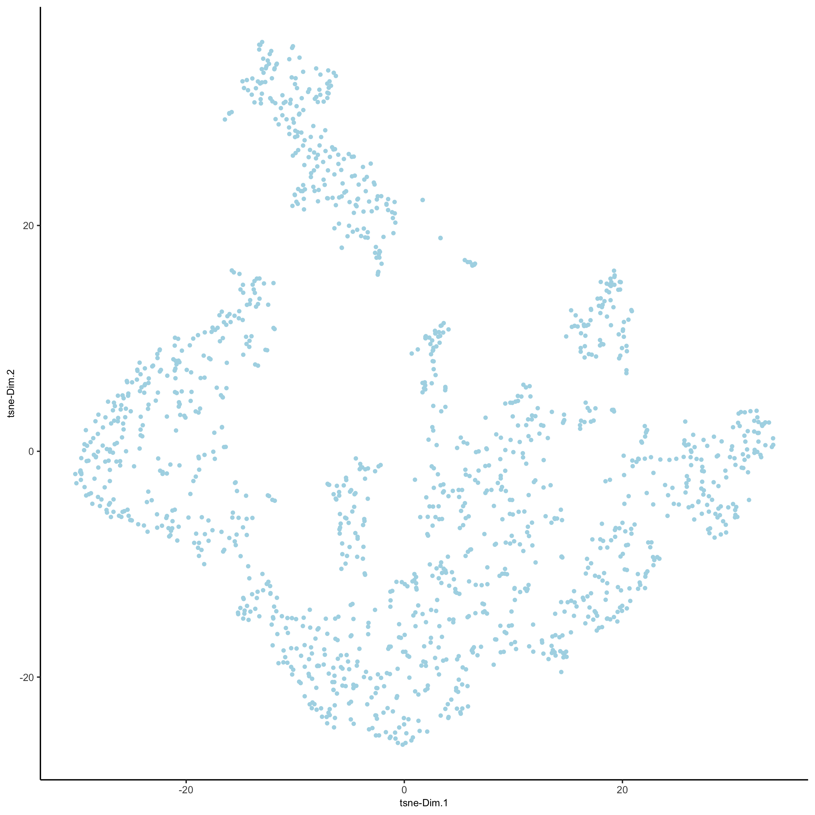
visium_kidney <- runtSNE(visium_kidney, dimensions_to_use = 1:10)
plotTSNE(gobject = visium_kidney,
    save_param = list(save_name = '3_e_tSNE_reduction'))

4. Clustering

## sNN network (default)
visium_kidney <- createNearestNetwork(gobject = visium_kidney, dimensions_to_use = 1:10, k = 15)
## Leiden clustering
visium_kidney <- doLeidenCluster(gobject = visium_kidney, resolution = 0.4, n_iterations = 1000)
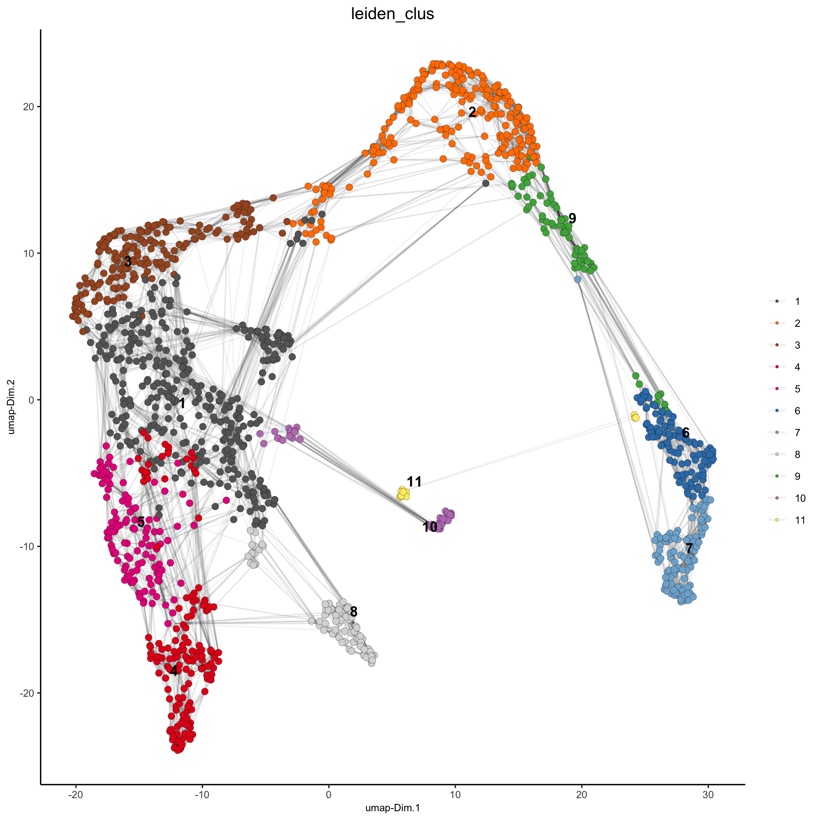
plotUMAP(gobject = visium_kidney,
    cell_color = 'leiden_clus', show_NN_network = T, point_size = 2.5,
    save_param = list(save_name = '4_a_UMAP_leiden'))

5. Co-Visualize

# expression and spatial
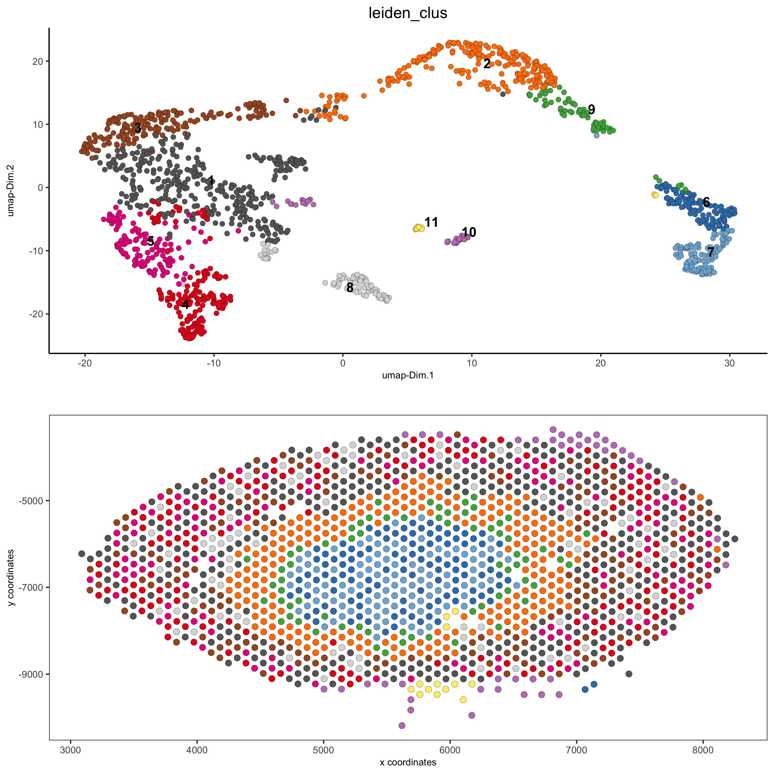
spatDimPlot(gobject = visium_kidney, cell_color = 'leiden_clus',
    dim_point_size = 2, spat_point_size = 2.5,
    save_param = list(save_name = '5_a_covis_leiden'))

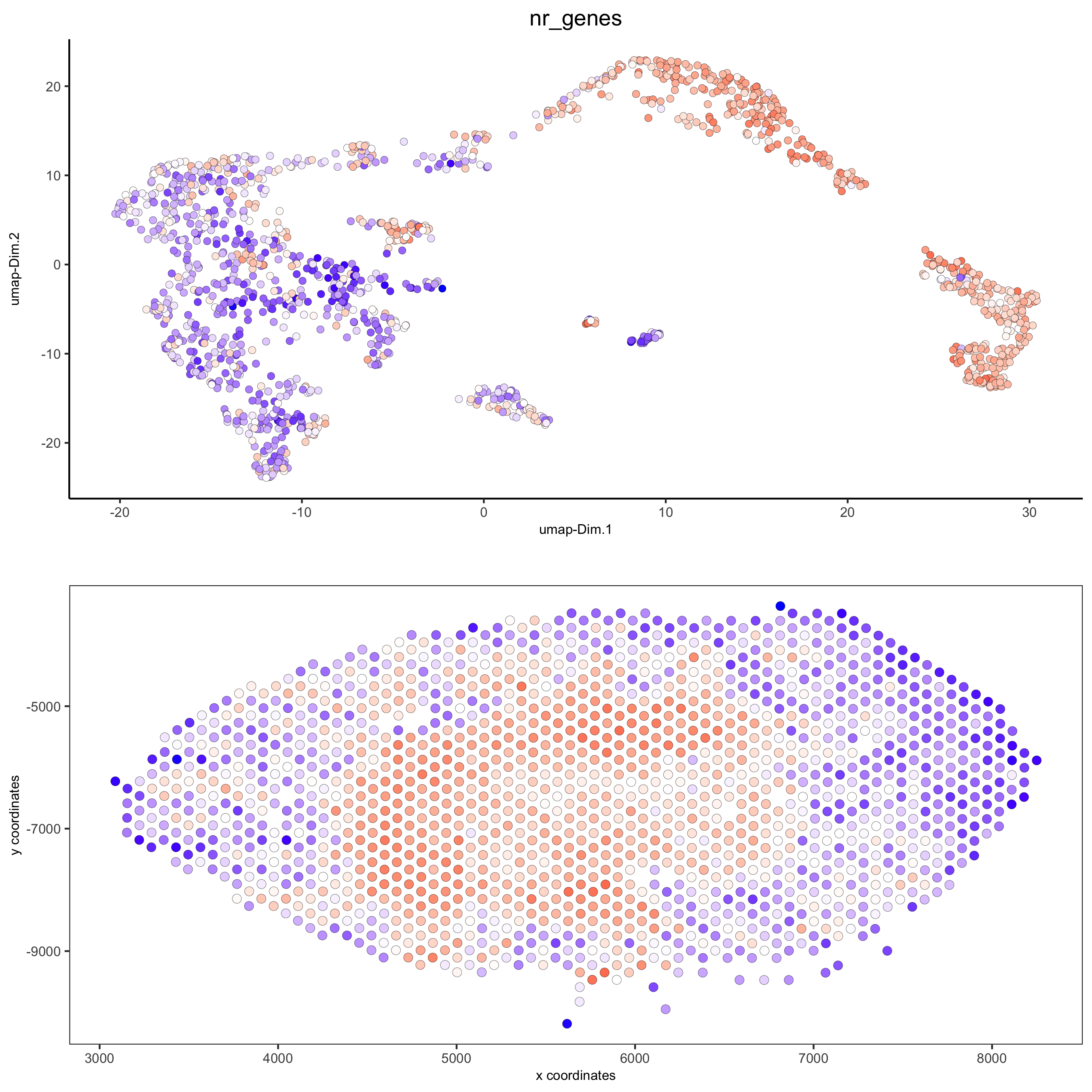
spatDimPlot(gobject = visium_kidney, cell_color = 'nr_genes', color_as_factor = F,
    dim_point_size = 2, spat_point_size = 2.5,
    save_param = list(save_name = '5_b_nr_genes'))

6. Cell-Type Marker Gene Detection

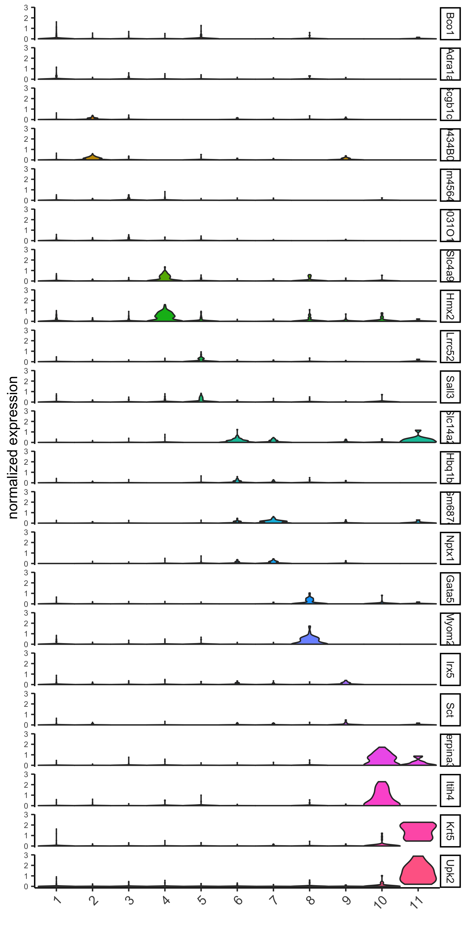
6.1 Gini

gini_markers_subclusters = findMarkers_one_vs_all(gobject = visium_kidney,
                      method = 'gini',
                      expression_values = 'normalized',
                      cluster_column = 'leiden_clus',
                      min_genes = 20,
                      min_expr_gini_score = 0.5,
                      min_det_gini_score = 0.5)
topgenes_gini = gini_markers_subclusters[, head(.SD, 2), by = 'cluster']$genes

# violinplot
violinPlot(visium_kidney, genes = unique(topgenes_gini), cluster_column = 'leiden_clus',
    strip_text = 8, strip_position = 'right',
    save_param = c(save_name = '6_a_violinplot_gini', base_width = 5, base_height = 10))

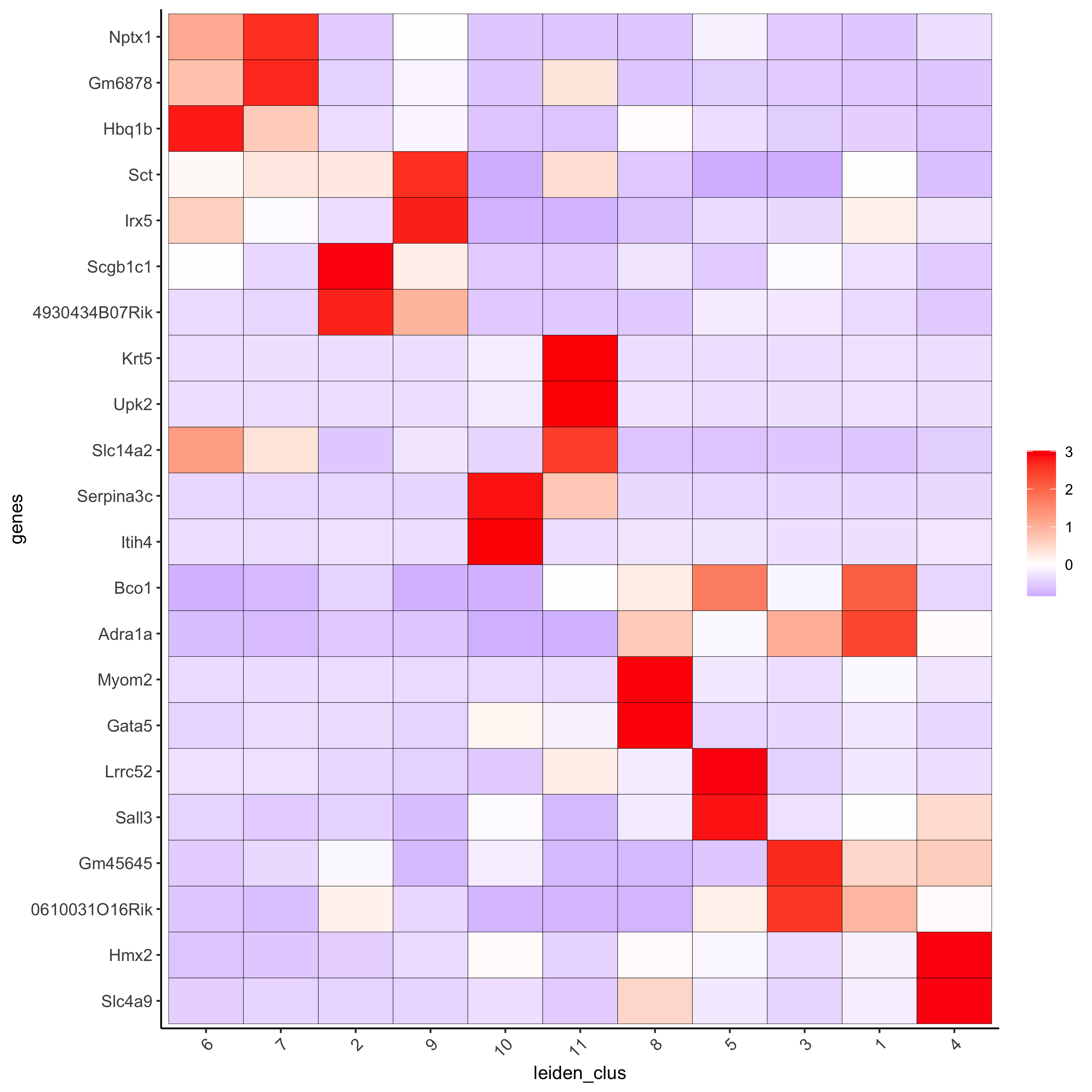
# cluster heatmap
plotMetaDataHeatmap(visium_kidney, selected_genes = topgenes_gini,
        metadata_cols = c('leiden_clus'),
        x_text_size = 10, y_text_size = 10,
        save_param = c(save_name = '6_b_metaheatmap_gini'))

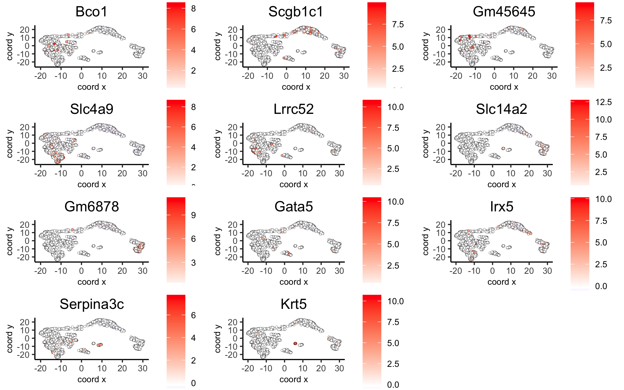
# umap plots
dimGenePlot2D(visium_kidney, expression_values = 'scaled',
      genes = gini_markers_subclusters[, head(.SD, 1), by = 'cluster']$genes,
      cow_n_col = 3, point_size = 1,
      save_param = c(save_name = '6_c_gini_umap', base_width = 8, base_height = 5))

6.2 Scran

scran_markers_subclusters = findMarkers_one_vs_all(gobject = visium_kidney,
                       method = 'scran',
                       expression_values = 'normalized',
                       cluster_column = 'leiden_clus')
topgenes_scran = scran_markers_subclusters[, head(.SD, 2), by = 'cluster']$genes

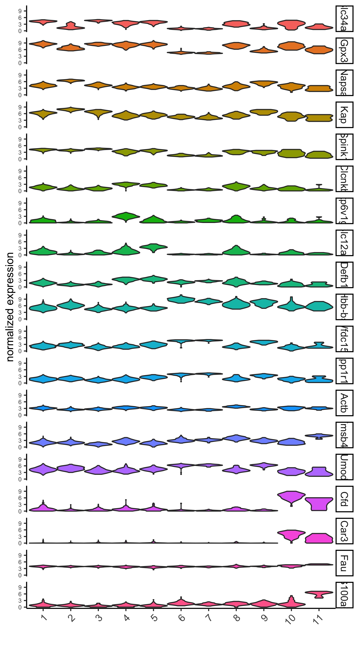
# violinplot
violinPlot(visium_kidney, genes = unique(topgenes_scran), cluster_column = 'leiden_clus',
    strip_text = 10, strip_position = 'right',
    save_param = c(save_name = '6_d_violinplot_scran', base_width = 5))

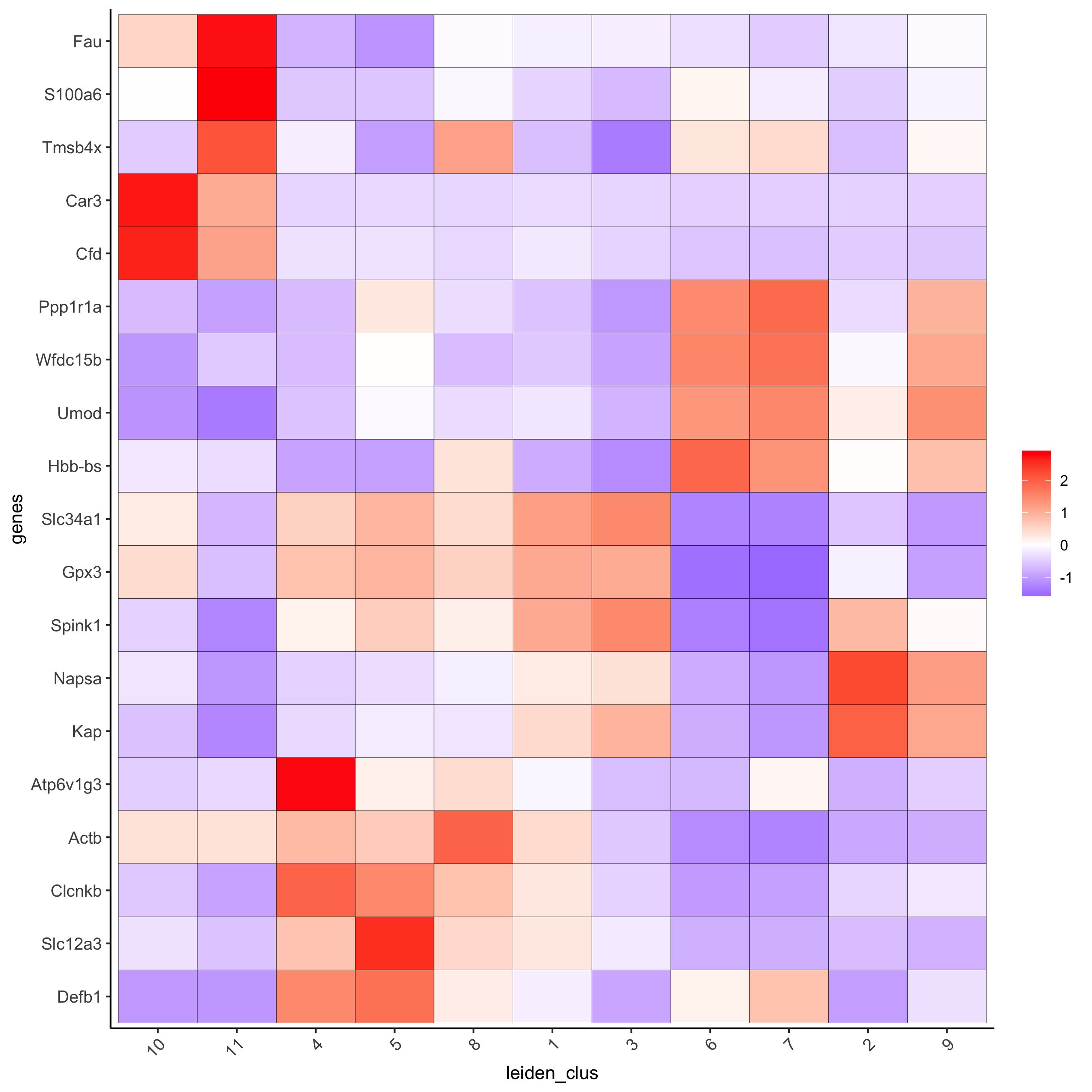
# cluster heatmap
lotMetaDataHeatmap(visium_kidney, selected_genes = topgenes_scran,
        metadata_cols = c('leiden_clus'),
        save_param = c(save_name = '6_e_metaheatmap_scran'))

# umap plots
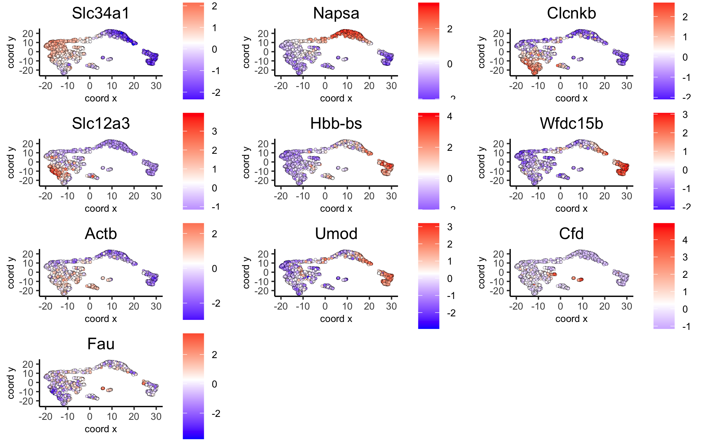
dimGenePlot(visium_kidney, expression_values = 'scaled',
    genes = scran_markers_subclusters[, head(.SD, 1), by = 'cluster']$genes,
    cow_n_col = 3, point_size = 1,
    save_param = c(save_name = '6_f_scran_umap', base_width = 8, base_height = 5))

7. Cell-Type Annotation

Visium spatial transcriptomics does not provide single-cell resolution, making cell type annotation a harder problem. Giotto provides 3 ways to calculate enrichment of specific cell-type signature gene list:

• PAGE

• RANK

• Hypergeometric Test

See the Mouse Visium Brain Dataset for an example.

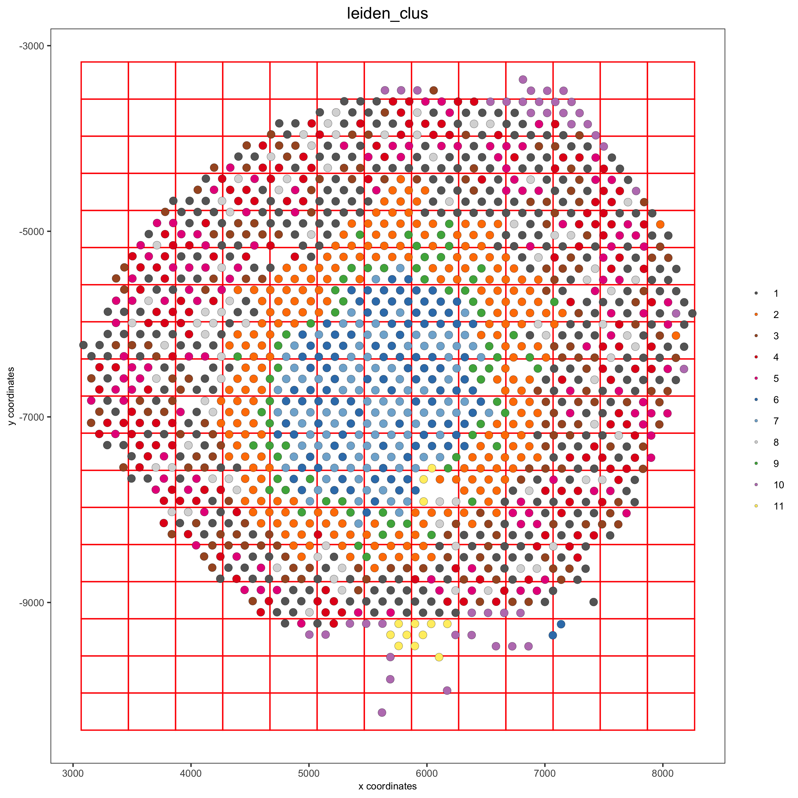
8. Spatial Grid

visium_kidney <- createSpatialGrid(gobject = visium_kidney,
               sdimx_stepsize = 400,
               sdimy_stepsize = 400,
               minimum_padding = 0)
spatPlot(visium_kidney, cell_color = 'leiden_clus', show_grid = T,
    grid_color = 'red', spatial_grid_name = 'spatial_grid',
    save_param = c(save_name = '8_grid'))

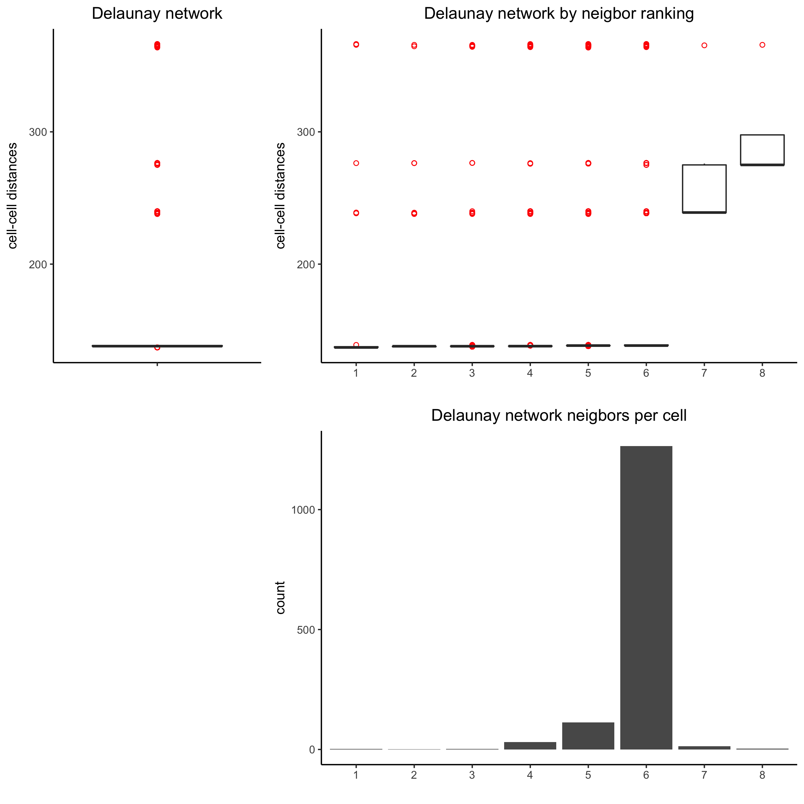
9. Spatial Network

## delaunay network: stats + creation
plotStatDelaunayNetwork(gobject = visium_kidney, maximum_distance = 400,
        save_param = c(save_name = '9_a_delaunay_network'))

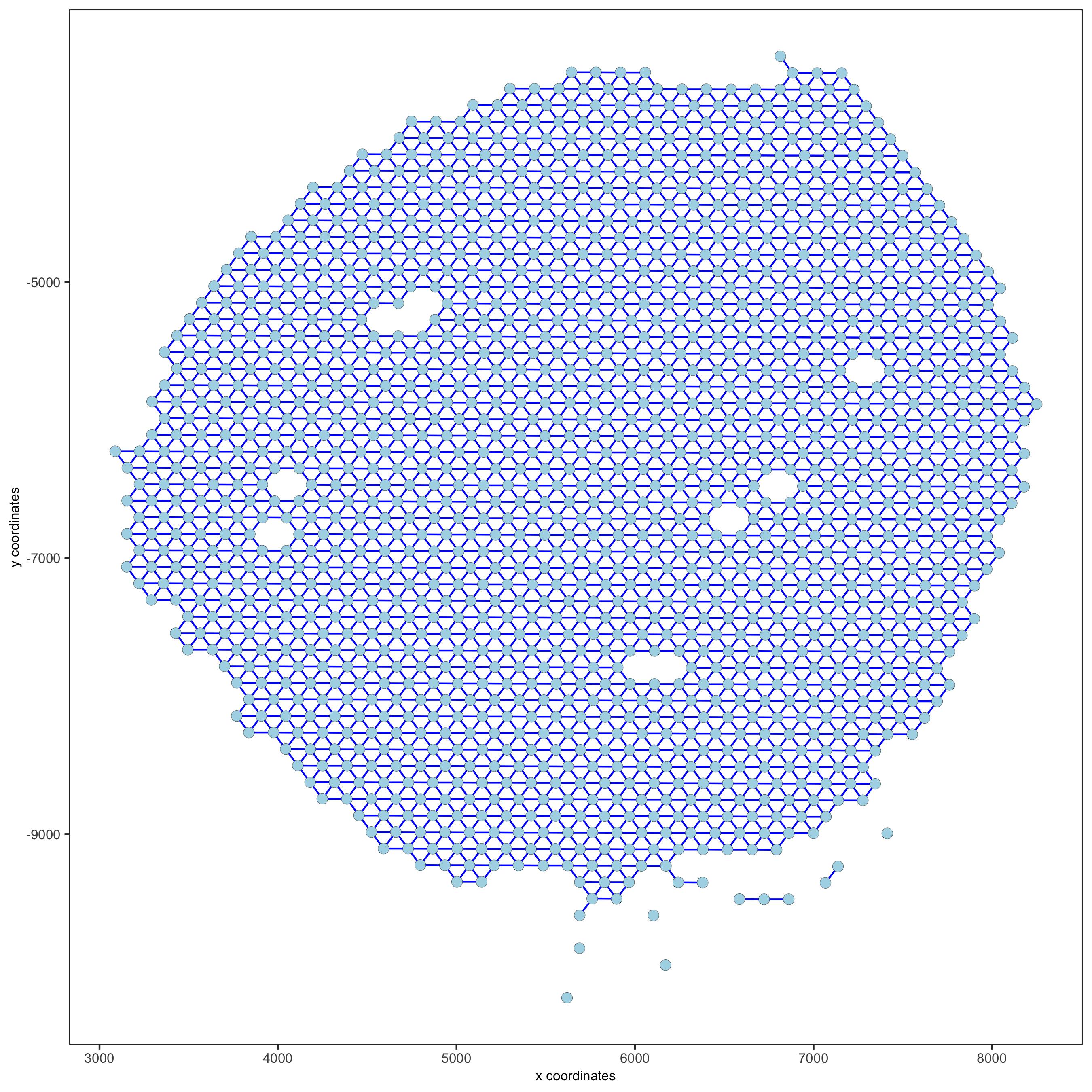
visium_kidney = createSpatialNetwork(gobject = visium_kidney, minimum_k = 0)
showNetworks(visium_kidney)
spatPlot(gobject = visium_kidney, show_network = T,
    network_color = 'blue', spatial_network_name = 'Delaunay_network',
    save_param = c(save_name = '9_b_delaunay_network'))

10. Spatial Genes and Co-Expression Patterns

10.1 Spatial Genes

## kmeans binarization
kmtest = binSpect(visium_kidney)
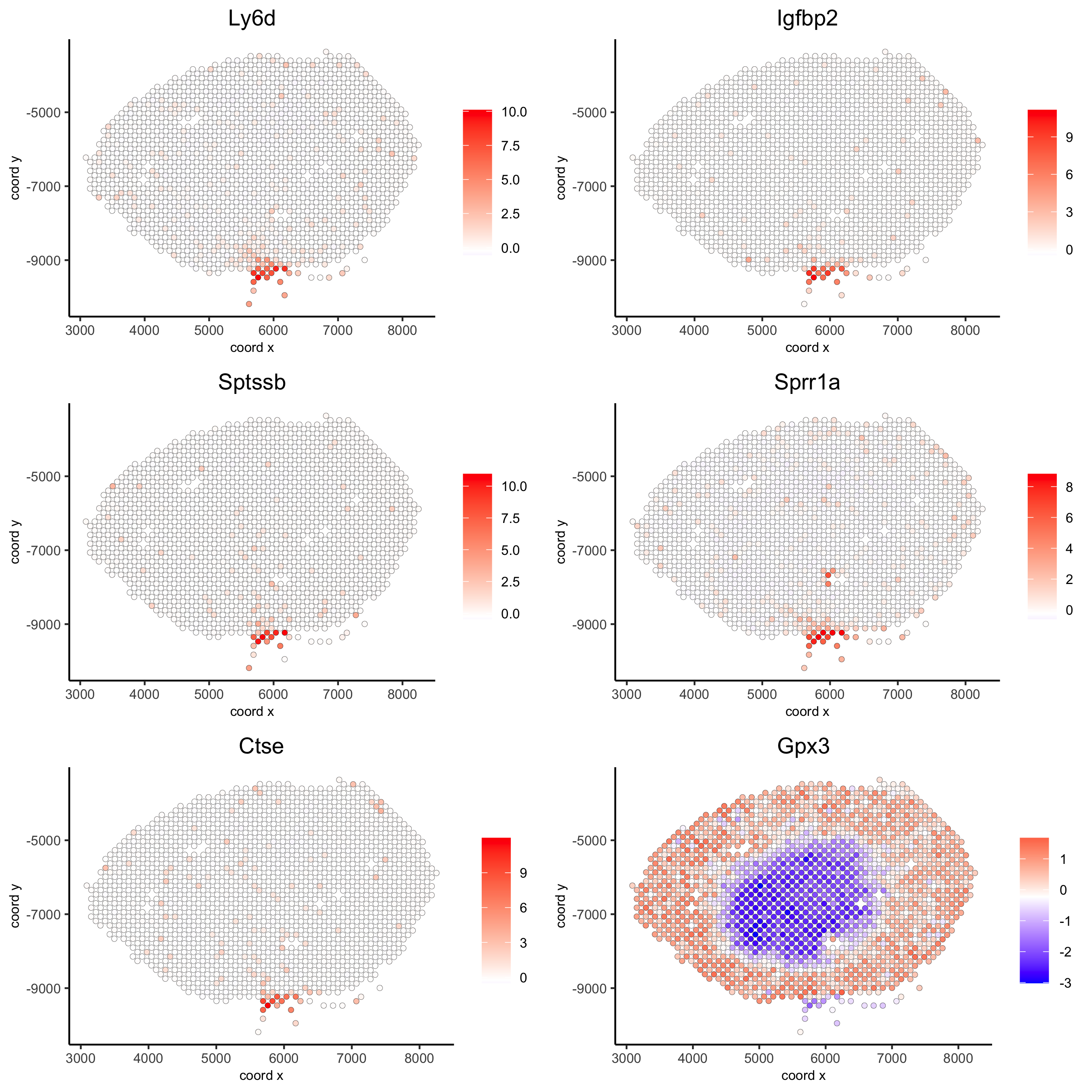
spatGenePlot(visium_kidney, expression_values = 'scaled',
     genes = kmtest$genes[1:6], cow_n_col = 2, point_size = 1.5,
     save_param = c(save_name = '10_a_spatial_genes_km'))

## rank binarization
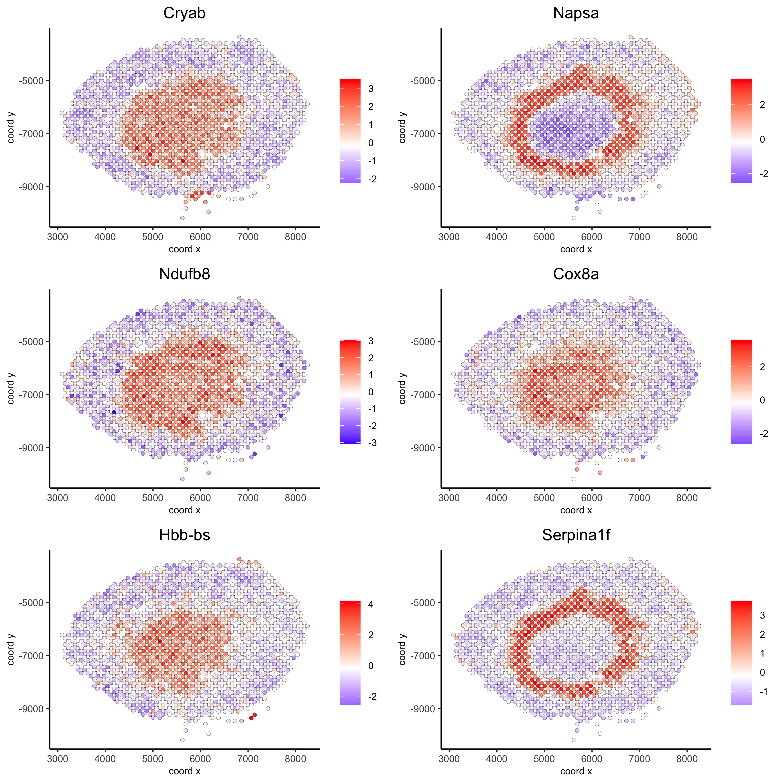
ranktest = binSpect(visium_kidney, bin_method = 'rank')
spatGenePlot(visium_kidney, expression_values = 'scaled',
     genes = ranktest$genes[1:6], cow_n_col = 2, point_size = 1.5,
     save_param = c(save_name = '10_b_spatial_genes_rank'))

10.2 Spatial Co-Expression Patterns

## spatially correlated genes ##
ext_spatial_genes = kmtest[1:500]$genes

# 1. calculate gene spatial correlation and single-cell correlation
# create spatial correlation object
spat_cor_netw_DT = detectSpatialCorGenes(visium_kidney,
                 method = 'network',
                 spatial_network_name = 'Delaunay_network',
                 subset_genes = ext_spatial_genes)

# 2. identify most similar spatially correlated genes for one gene
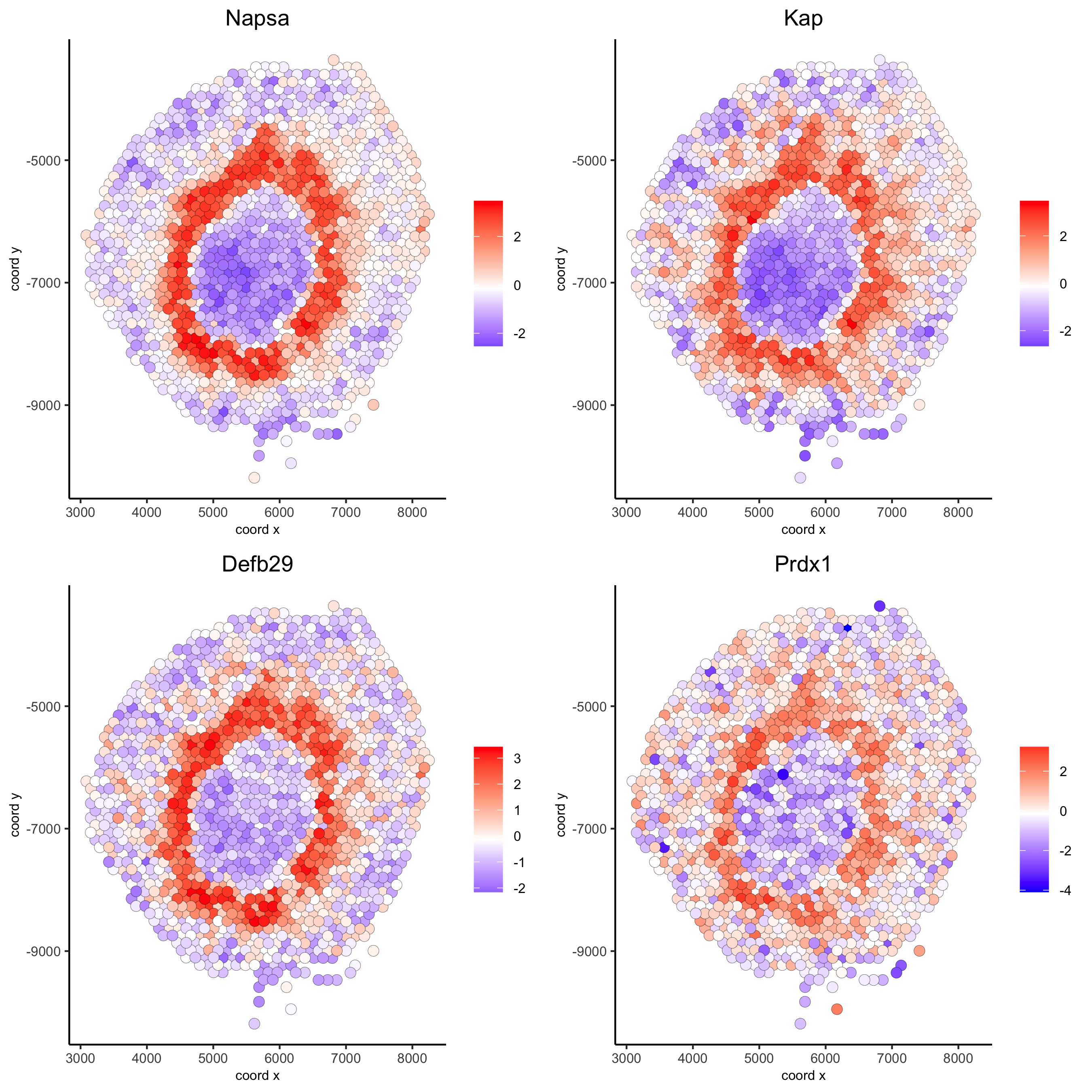
Napsa_top10_genes = showSpatialCorGenes(spat_cor_netw_DT, genes = 'Napsa', show_top_genes = 10)
spatGenePlot(visium_kidney, expression_values = 'scaled',
     genes = c('Napsa', 'Kap', 'Defb29', 'Prdx1'), point_size = 3,
     save_param = c(save_name = '10_d_Napsa_correlated_genes'))

# 3. cluster correlated genes & visualize
spat_cor_netw_DT = clusterSpatialCorGenes(spat_cor_netw_DT, name = 'spat_netw_clus', k = 8)

heatmSpatialCorGenes(visium_kidney, spatCorObject = spat_cor_netw_DT, use_clus_name = 'spat_netw_clus',
         save_param = c(save_name = '10_e_heatmap_correlated_genes', save_format = 'pdf',
                base_height = 6, base_width = 8, units = 'cm'),
         heatmap_legend_param = list(title = NULL))

# 4. rank spatial correlated clusters and show genes for selected clusters
netw_ranks = rankSpatialCorGroups(visium_kidney, spatCorObject = spat_cor_netw_DT, use_clus_name = 'spat_netw_clus',
              save_param = c(save_name = '10_f_rank_correlated_groups',
                     base_height = 3, base_width = 5))

top_netw_spat_cluster = showSpatialCorGenes(spat_cor_netw_DT, use_clus_name = 'spat_netw_clus',
                    selected_clusters = 6, show_top_genes = 1)

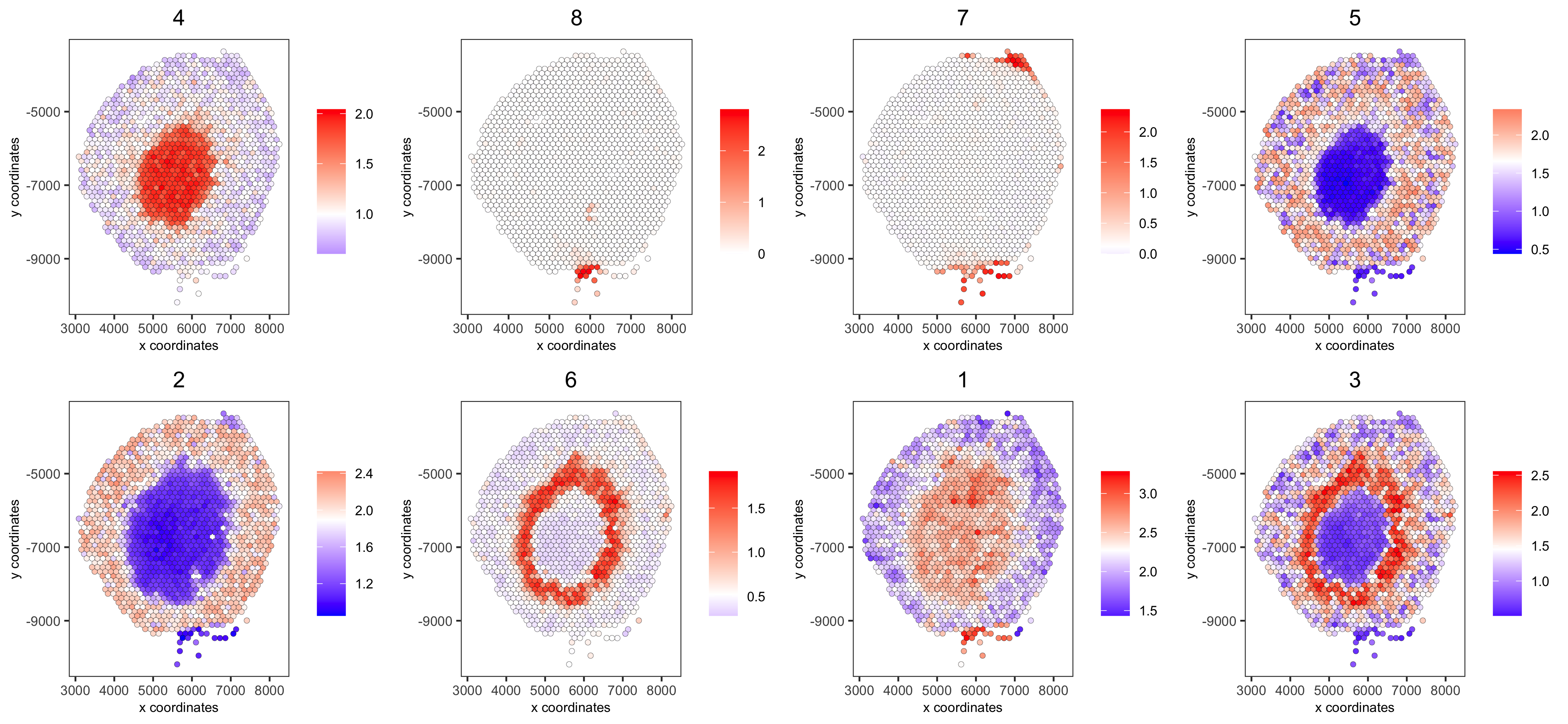
# 5. create metagene enrichment score for clusters
cluster_genes_DT = showSpatialCorGenes(spat_cor_netw_DT, use_clus_name = 'spat_netw_clus', show_top_genes = 1)
cluster_genes = cluster_genes_DT$clus; names(cluster_genes) = cluster_genes_DT$gene_ID

visium_kidney = createMetagenes(visium_kidney, gene_clusters = cluster_genes, name = 'cluster_metagene')

spatCellPlot(visium_kidney,
     spat_enr_names = 'cluster_metagene',
     cell_annotation_values = netw_ranks$clusters,
     point_size = 1.5, cow_n_col = 4,
     save_param = c(save_name = '10_g_spat_enrichment_score_plots',
            base_width = 13, base_height = 6))

# example for gene per cluster
top_netw_spat_cluster = showSpatialCorGenes(spat_cor_netw_DT, use_clus_name = 'spat_netw_clus',
                    selected_clusters = 1:8, show_top_genes = 1)
first_genes = top_netw_spat_cluster[, head(.SD, 1), by = clus]$gene_ID
cluster_names = top_netw_spat_cluster[, head(.SD, 1), by = clus]$clus
names(first_genes) = cluster_names
first_genes = first_genes[as.character(netw_ranks$clusters)]

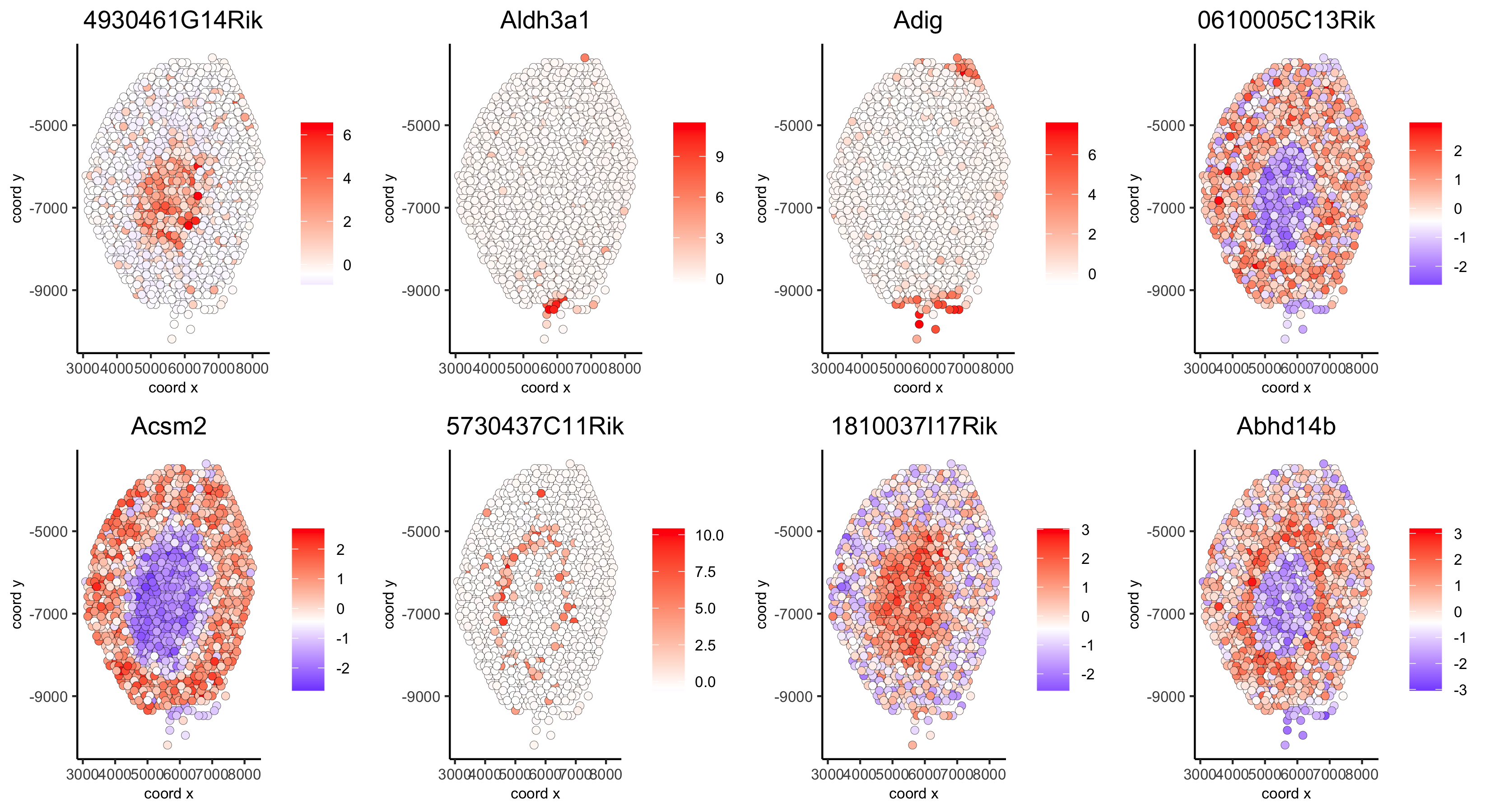
spatGenePlot(visium_kidney, genes = first_genes, expression_values = 'scaled', cow_n_col = 4, midpoint = 0, point_size = 2,
     save_param = c(save_name = '10_h_spat_enrichment_score_plots_genes',
            base_width = 11, base_height = 6))

11. HMRF Domains

# HMRF requires a fully connected network!
visium_kidney = createSpatialNetwork(gobject = visium_kidney, minimum_k = 2, name = 'Delaunay_full')

# spatial genes
my_spatial_genes <- kmtest[1:100]$genes

# do HMRF with different betas
hmrf_folder = paste0(results_folder,'/','11_HMRF/')
if(!file.exists(hmrf_folder)) dir.create(hmrf_folder, recursive = T)

HMRF_spatial_genes = doHMRF(gobject = visium_kidney, expression_values = 'scaled',
            spatial_network_name = 'Delaunay_full',
            spatial_genes = my_spatial_genes,
            k = 5,
            betas = c(0, 1, 6),
            output_folder = paste0(hmrf_folder, '/', 'Spatial_genes/SG_topgenes_k5_scaled'))

## view results of HMRF
for(i in seq(0, 5, by = 1)) {
    viewHMRFresults2D(gobject = visium_kidney,
        HMRFoutput = HMRF_spatial_genes,
        k = 5, betas_to_view = i,
        point_size = 2)
}

Alternative Way to View Results

#results = writeHMRFresults(gobject = ST_test,
#                           HMRFoutput = HMRF_spatial_genes,
#                           k = 5, betas_to_view = seq(0, 25, by = 5))
#ST_test = addCellMetadata(ST_test, new_metadata = results, by_column = T, column_cell_ID = 'cell_ID')


## add HMRF of interest to giotto object
visium_kidney = addHMRF(gobject = visium_kidney,
        HMRFoutput = HMRF_spatial_genes,
        k = 5, betas_to_add = c(0, 2),
        hmrf_name = 'HMRF')

## visualize
spatPlot(gobject = visium_kidney, cell_color = 'HMRF_k5_b.0', point_size = 5,
    save_param = c(save_name = '11_a_HMRF_k5_b.0'))

spatPlot(gobject = visium_kidney, cell_color = 'HMRF_k5_b.2', point_size = 5,
    save_param = c(save_name = '11_b_HMRF_k5_b.2'))

Export and Create Giotto Viewer

# check which annotations are available
combineMetadata(visium_kidney)

# select annotations, reductions and expression values to view in Giotto Viewer
viewer_folder = paste0(results_folder, '/', 'mouse_visium_kidney_viewer')

exportGiottoViewer(gobject = visium_kidney,
       output_directory = viewer_folder,
       spat_enr_names = 'PAGE',
       factor_annotations = c('in_tissue',
                  'leiden_clus'),
       numeric_annotations = c('nr_genes',
                   'clus_25'),
       dim_reductions = c('tsne', 'umap'),
       dim_reduction_names = c('tsne', 'umap'),
       expression_values = 'scaled',
       expression_rounding = 2,
       overwrite_dir = T)