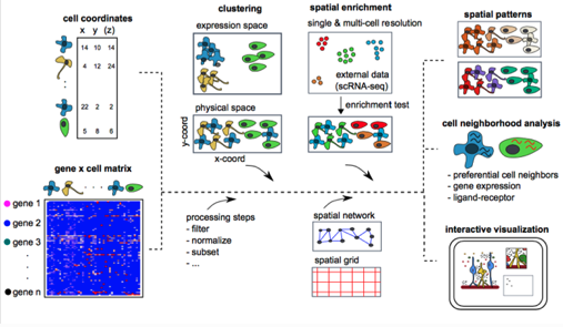
Giotto Workflow
Workflow Diagram
0. Optional: Install a Giotto Environment
To perform all potential steps and analysis in the Giotto spatial toolbox the user needs to have a number of python modules installed. To make this process as flexible and easy as possible two different strategies can be used. See the Part 2.2 Giotto-Specific Python Packages for more detailed information on installing Giotto and all of the required modules needed to use Giotto succesffully.
The user can install all the necessary modules themself and then proivide the path to their python or environment (e.g. Conda) as an instruction.
library(Giotto)
my_instructions = createGiottoInstructions(python_path = 'your/python/path')
my_giotto_object = createGiottoObject(raw_exprs = '...',
                  spatial_locs = '...',
                  instructions = my_instructions)
Alternatively, the user can just install a giotto python environment using r-miniconda. This was the method that was implemented in the reticulate package. In this case the environment will be automatically detected and no specific python path need to be provided. The installation, re-installation and removal is explained in futher detail below.
Load Giotto into R
library(Giotto)
Install Giotto Environment
installGiottoEnvironment()
Re-install the Giotto Environment
installGiottoEnvironment(force_environment = TRUE)
Re-install mini-conda and Giotto Environment
installGiottoEnvironment(force_miniconda = TRUE)
Remove Giotto Environment
removeGiottoEnvironment()
1. Create a Giotto Object
Minimum Requirements
Expression Matrix
Spatial Locations
library(Giotto)

# 1. Directly from the file paths
path_to_matrix = system.file("extdata", "seqfish_field_expr.txt", package = 'Giotto')
path_to_locations = system.file("extdata", "seqfish_field_locs.txt", package = 'Giotto')

my_giotto_object = createGiottoObject(raw_exprs = path_to_matrix,
                  spatial_locs = path_to_locations)


# 2. Use an existing matrix and data.table
expression_matrix = readExprMatrix(path_to_matrix) # fast method to read expression matrix
cell_locations = data.table::fread(path_to_locations)

my_giotto_object = createGiottoObject(raw_exprs = expression_matrix,
                  spatial_locs = cell_locations)
Additional Features
Previously obtained information can be provided using any of the function parameters to add:
Cell or gene metadata
Spatial networks or grids
Dimensions reduction
Giotto images
Offset file
Instructions
Usually specifying your own instructions can be most useful to:
Specify a python path
Determining the outputs of plots
Automatically saving plots to particular directories
library(Giotto)

# 1. Directly use a path
path_to_matrix = system.file("extdata", "seqfish_field_expr.txt", package = 'Giotto')
path_to_locations = system.file("extdata", "seqfish_field_locs.txt", package = 'Giotto')

# 2. Create your own instructions
path_to_python = '/usr/bin/python3' # can be something else
working_directory = getwd() # this will use your current working directory
my_instructions = createGiottoInstructions(python_path = path_to_python,
                   save_dir = working_directory)

# 3. Create your giotto object
my_giotto_object = createGiottoObject(raw_exprs = path_to_matrix,
                  spatial_locs = path_to_locations,
                  cell_metadata = my_cell_metadata,
                  gene_metadata = my_gene_metadata,
                  instructions = my_instructions)

# 4. Check which giotto instructions are associated with your giotto object
showGiottoInstructions(my_giotto_object)
2. Process and Filter a Giotto Object
Load Giotto into R
library(Giotto)
2.1 Create a Giotto object
path_to_matrix = system.file("extdata", "seqfish_field_expr.txt", package = 'Giotto')
path_to_locations = system.file("extdata", "seqfish_field_locs.txt", package = 'Giotto')
my_giotto_object = createGiottoObject(raw_exprs = path_to_matrix,
                  spatial_locs = path_to_locations)
2.2 Filter Giotto object based on gene and cell coverage
my_giotto_object <- filterGiotto(gobject = my_giotto_object,
             expression_threshold = 1,
             gene_det_in_min_cells = 10,
             min_det_genes_per_cell = 5)
2.3 Normalize Giotto object
my_giotto_object <- normalizeGiotto(gobject = my_giotto_object, scalefactor = 6000, verbose = T)
2.4 Optional: Add gene and cell statistics and adjust matrix for technical covariates or batch effects
my_giotto_object <- addStatistics(gobject = my_giotto_object)
my_giotto_object <- adjustGiottoMatrix(gobject = my_giotto_object,
                   expression_values = c('normalized'),
                   covariate_columns = c('nr_genes', 'total_expr'))
3. Dimension Reduction
Load Giotto into R
library(Giotto)
3.1 Create and process Giotto object
path_to_matrix = system.file("extdata", "seqfish_field_expr.txt", package = 'Giotto')
path_to_locations = system.file("extdata", "seqfish_field_locs.txt", package = 'Giotto')
my_giotto_object = createGiottoObject(raw_exprs = path_to_matrix,
                  spatial_locs = path_to_locations)
my_giotto_object <- filterGiotto(gobject = my_giotto_object)
my_giotto_object <- normalizeGiotto(gobject = my_giotto_object)
3.2 Highly variable genes
my_giotto_object <- calculateHVG(gobject = my_giotto_object)
3.3 PCA
# Run PCA
my_giotto_object <- runPCA(gobject = my_giotto_object)

# Identify most informative principal components
screePlot(my_giotto_object, ncp = 20)
jackstrawPlot(my_giotto_object, ncp = 20)
3.4 UMAP & TSNE
# UMAP
my_giotto_object <- runUMAP(my_giotto_object, dimensions_to_use = 1:5)
plotUMAP(gobject = my_giotto_object)

# TSNE
my_giotto_object <- runtSNE(my_giotto_object, dimensions_to_use = 1:5)
plotTSNE(gobject = my_giotto_object)

# plot PCA results
plotPCA(my_giotto_object)
4. Cluster cells or spots
4.1 Processing steps
Load Giotto into R
library(Giotto)
path_to_matrix = system.file("extdata", "seqfish_field_expr.txt", package = 'Giotto')
path_to_locations = system.file("extdata", "seqfish_field_locs.txt", package = 'Giotto')

my_giotto_object = createGiottoObject(raw_exprs = path_to_matrix,
                  spatial_locs = path_to_locations)

# processing
my_giotto_object <- filterGiotto(gobject = seqfish_mini,
             expression_threshold = 0.5,
             gene_det_in_min_cells = 20,
             min_det_genes_per_cell = 0)
my_giotto_object <- normalizeGiotto(gobject = my_giotto_object)

# dimension reduction
my_giotto_object <- calculateHVG(gobject = my_giotto_object)
my_giotto_object <- runPCA(gobject = my_giotto_object)
my_giotto_object <- runUMAP(my_giotto_object, dimensions_to_use = 1:5)
4.2 Clustering
4.2.1 Clustering algorithms
Giotto provides a number of different clustering algorithms, here we show some of the most popular.
# Leiden
my_giotto_object = doLeidenCluster(my_giotto_object, name = 'leiden_clus')
plotUMAP_2D(my_giotto_object, cell_color = 'leiden_clus', point_size = 3)

# Louvain
my_giotto_object = doLouvainCluster(my_giotto_object, name = 'louvain_clus')
plotUMAP_2D(my_giotto_object, cell_color = 'louvain_clus', point_size = 3)

# K-means
my_giotto_object = doKmeans(my_giotto_object, centers = 4, name = 'kmeans_clus')
plotUMAP_2D(my_giotto_object, cell_color = 'kmeans_clus', point_size = 3)

# Hierarchical
my_giotto_object = doHclust(my_giotto_object, k = 4, name = 'hier_clus')
plotUMAP_2D(my_giotto_object, cell_color = 'hier_clus', point_size = 3)
4.2.2 Clustering similarity and merging
To fine-tune clustering results Giotto provides methods to calculate similarities between clusters and merge clusters based on correlation and size parameters.
# Calculate cluster similarities to see how individual clusters are correlated
cluster_similarities = getClusterSimilarity(my_giotto_object,
                    cluster_column = 'leiden_clus')

# Merge similar clusters based on correlation and size parameters
mini_giotto_single_cell = mergeClusters(my_giotto_object,
                cluster_column = 'leiden_clus',
                min_cor_score = 0.7,
                force_min_group_size = 4)

# Visualize
pDataDT(my_giotto_object)
plotUMAP_2D(my_giotto_object, cell_color = 'merged_cluster', point_size = 3)
4.3 Dendrogram splits
A dendrogram can be created from the clustering results. This may for example help in identifying genes that are most differentially expressed between branches.
splits = getDendrogramSplits(my_giotto_object, cluster_column = 'merged_cluster')
4.4 Subclustering See seqfish+ clustering example.
5. Identify differentially expressed genes
Marker Gene Detection
Load Giotto into R
library(Giotto)
data("mini_giotto_single_cell")
This tutorial starts from a pre-computed mini Giotto object, which has already undergone pre-processing, dimensions reduction and clustering steps. Currently provides 3 different methods to identify marker genes: * using a new Gini-index method * using Scran * using Mast
Each method can either identify marker genes between 2 selected (groups of) clusters or for each individual cluster.
5.1 Gini
# Between 2 groups
gini_markers = findGiniMarkers(gobject = mini_giotto_single_cell,
               cluster_column = 'leiden_clus',
               group_1 = 1,
               group_2 = 2)
# For each cluster
gini_markers = findGiniMarkers_one_vs_all(gobject = mini_giotto_single_cell,
                  cluster_column = 'leiden_clus')
5.2 Scran
Requires Scran to be installed.
# Between 2 groups
scran_markers = findScranMarkers(gobject = mini_giotto_single_cell,
             cluster_column = 'leiden_clus',
             group_1 = 1,
             group_2 = 2)
# For each cluster
scran_markers = findScranMarkers_one_vs_all(gobject = mini_giotto_single_cell,
                    cluster_column = 'leiden_clus')
5.3 Mast
Requires Mast to be installed.
# Between 2 groups
mast_markers = findMastMarkers(gobject = mini_giotto_single_cell,
            cluster_column = 'leiden_clus',
            group_1 = 1,
            group_2 = 2)

# For each cluster
mast_markers = findMastMarkers_one_vs_all(gobject = mini_giotto_single_cell,
                  cluster_column = 'leiden_clus')
5.4 Wrapper
A general wrapper has also been created which covers all three methods. See findMarkers and findMarkers_one_vs_all and specify the method parameter.
6. Annotate clusters
Giotto Annotation Tools
Load Giotto into R
library(Giotto)
data("mini_giotto_single_cell")
Clustering results or other type of metadata information can be further annotated by the user by providing a named vector. Cell or gene metadata can also be removed from the Giotto object if required.
6.1 Annotate clusters or other type of metadata information
# Show leiden clustering results
cell_metadata = pDataDT(mini_giotto_single_cell)
cell_metadata[['leiden_clus']]

# Create vector with cell type names as names of the vector
clusters_cell_types = c('cell_type_1', 'cell_type_2', 'cell_type_3')
names(clusters_cell_types) = 1:3 # leiden clustering results

# Convert cluster results into annotations and add to cell metadata
mini_giotto_single_cell = annotateGiotto(gobject = mini_giotto_single_cell,
                 annotation_vector = clusters_cell_types,
                 cluster_column = 'leiden_clus',
                 name = 'cell_types2')
# Inspect new annotation column
pDataDT(mini_giotto_single_cell)

# Visualize annotation results
# Annotation name is cell_types2 as provided in the previous command
spatDimPlot(gobject = mini_giotto_single_cell,
    cell_color = 'cell_types2',
    spat_point_size = 3, dim_point_size = 3)
6.2 Remove cell annotation
# Show cell metadata
pDataDT(mini_giotto_single_cell)

# Remove cell_types column
mini_giotto_single_cell = removeCellAnnotation(mini_giotto_single_cell,
                       columns = 'cell_types')
6.3 Remove gene annotation
# Show gene metadata
fDataDT(mini_giotto_single_cell)

# Remove nr_cells column
mini_giotto_single_cell = removeGeneAnnotation(mini_giotto_single_cell,
                    columns = 'nr_cells')
7. Cell-type enrichment or deconvolution per spot
Giotto spot enrichment tools
Not yet available. Check out the visium brain datasets for examples.
7.1 Processing steps
Load Giotto into R
library(Giotto)
path_to_matrix = system.file("extdata", "visium_DG_expr.txt.gz", package = 'Giotto')
path_to_locations = system.file("extdata", "visium_DG_locs.txt", package = 'Giotto')

my_giotto_object = createGiottoObject(raw_exprs = path_to_matrix,
                  spatial_locs = path_to_locations)

# processing
my_giotto_object <- normalizeGiotto(gobject = my_giotto_object)
7.2 Run spatial cell type enrichments methods
7.2.1 PAGE Enrichment
astro_epen_markers = c("Krt15" , "Apoc1" , "Igsf1" , "Gjb6" , "Slc26a3" ,
           "1500015O10Rik" , "S1pr1" , "Riiad1" , "Cldn10" , "Itih3" ,
           "Ccdc153" , "Cbs" , "C4b" , "Gm11627" , "Folr1" ,
           "Calml4" , "Aqp4" , "Ppp1r3g" , "1700012B09Rik" , "Hes5")

gran_markers = c("Nr3c2", "Gabra5", "Tubgcp2", "Ahcyl2",
     "Islr2", "Rasl10a", "Tmem114", "Bhlhe22",
     "Ntf3", "C1ql2")

cortex_hippo_markers = c("6330403A02Rik" , "Tekt5" , "Wipf3" , "1110032F04Rik" , "Lmo3" ,
         "Nrep" , "Slc30a3" , "Plcxd2" , "D630023F18Rik" , "Nptx1" ,
         "C1ql3" , "Ddit4l" , "Fezf2" , "Col24a1" , "Kcnf1" ,
         "Tnnc1" , "Gm12371" , "3110035E14Rik" , "Nr4a2" , "Nr4a3")

oligo_markers = c("Efhd1" , "H2-Ab1" , "Enpp6" , "Ninj2" , "Bmp4" ,
      "Tnr" , "Hapln2" , "Neu4" , "Wfdc18" , "Ccp110" ,
      "Gm26834" , "Il23a" , "Arap2" , "Nkx2-9" , "Mal" ,
      "Tmem2" , "Birc2" , "Cdkn1c" , "Pak4" , "Tmem88b")


signature_matrix = makeSignMatrixPAGE(sign_names = c('Astro_ependymal',
                         'Granule',
                         'Cortex_hippocampus',
                         'Oligo_dendrocytes'),
                  sign_list = list(astro_epen_markers,
                           gran_markers,
                           cortex_hippo_markers,
                           oligo_markers))

# runSpatialEnrich() can also be used as a wrapper for all currently provided enrichment options
my_giotto_object = runPAGEEnrich(gobject = my_giotto_object,
             sign_matrix = signature_matrix,
             min_overlap_genes = 2)
cell_types_subset = colnames(signature_matrix)
spatCellPlot(gobject = my_giotto_object,
     spat_enr_names = 'PAGE',
     cell_annotation_values = cell_types_subset,
     cow_n_col = 2,coord_fix_ratio = NULL, point_size = 2.75)
7.2.2 RANK Enrichment
# Single-cell RNA-seq data from Zeisel et al
# Mini data is available at https://github.com/RubD/spatial-datasets/tree/master/data/2019_visium_brain

# Single cell matrix
single_cell_DT = fread('/path/to/raw_exp_small.txt')
single_cell_matrix = Giotto:::dt_to_matrix(single_cell_DT)
single_cell_matrix[1:4, 1:4]

# Single cell annotation vector
cell_annotations = read.table(file = '/path/to/major_cluster_small.txt')
cell_annotations = as.vector(cell_annotations$V1)
cell_annotations[1:10]

# 1.2 create rank matrix
rank_matrix = makeSignMatrixRank(sc_matrix = single_cell_matrix, sc_cluster_ids = cell_annotations)


# 1.3 enrichment test with RANK
# runSpatialEnrich() can also be used as a wrapper for all currently provided enrichment options
my_giotto_object = runRankEnrich(gobject = my_giotto_object, sign_matrix = rank_matrix)

cell_types_subset = c("Astro_ependymal", "Oligo_dendrocyte" , "Cortex_hippocampus" , "Granule_neurons" )
spatCellPlot(gobject = my_giotto_object,
     spat_enr_names = 'rank',
     cell_annotation_values = cell_types_subset,
     cow_n_col = 3,coord_fix_ratio = NULL, point_size = 1.75)
7.2.3 Hypergeometric enrichment
my_giotto_object = runHyperGeometricEnrich(gobject = my_giotto_object,
                   sign_matrix = signature_matrix)

cell_types_subset = colnames(signature_matrix)
spatCellPlot(gobject = my_giotto_object,
     spat_enr_names = 'hypergeometric',
     cell_annotation_values = cell_types_subset,
     cow_n_col = 2,coord_fix_ratio = NULL, point_size = 2.75)
7.2.4 Deconvolution
my_giotto_object = runDWLSDeconv(gobject = my_giotto_object, sign_matrix = signature_matrix)
8. Create a Spatial grid or Network
Load Giotto into R
library(Giotto)
data("mini_giotto_single_cell")
8.1 Create a spatial grid
mini_giotto_single_cell <- createSpatialGrid(gobject = mini_giotto_single_cell,
                    sdimx_stepsize = 250,
                    sdimy_stepsize = 250,
                    minimum_padding = 50)
# Visualize grid
spatPlot(gobject = mini_giotto_single_cell, show_grid = T, point_size = 1.5)

# Create another larger grid
mini_giotto_single_cell <- createSpatialGrid(gobject = mini_giotto_single_cell,
                    sdimx_stepsize = 350,
                    sdimy_stepsize = 350,
                    minimum_padding = 50,
                    name = 'large_grid')

# Show available grids
showGrids(mini_giotto_single_cell)

# Visualize other grid
spatPlot2D(gobject = mini_giotto_single_cell, point_size = 1.5,
   show_grid = T, spatial_grid_name = 'large_grid')
8.2 Create a spatial network
# Get information about the Delaunay network
plotStatDelaunayNetwork(gobject = mini_giotto_single_cell, maximum_distance = 400)

# Create a spatial network, the Delaunay network is the default network
# Default name = 'Delaunay_network'
mini_giotto_single_cell = createSpatialNetwork(gobject = mini_giotto_single_cell, minimum_k = 2,
                maximum_distance_delaunay = 400)

# Create a kNN network with 4 spatial neighbors
# Default name = 'kNN_network'
mini_giotto_single_cell = createSpatialNetwork(gobject = mini_giotto_single_cell, minimum_k = 2,
                method = 'kNN', k = 4)

# Show available networks
showNetworks(mini_giotto_single_cell)

# Visualize the two different spatial networks
spatPlot(gobject = mini_giotto_single_cell, show_network = T,
 network_color = 'blue', spatial_network_name = 'Delaunay_network',
 point_size = 2.5, cell_color = 'cell_types')

spatPlot(gobject = mini_giotto_single_cell, show_network = T,
 network_color = 'blue', spatial_network_name = 'kNN_network',
 point_size = 2.5, cell_color = 'cell_types')
9. Find genes with a spatially coherent gene expression pattern
Spatial Gene Detection Tools
Load Giotto into R
library(Giotto)
9.1 Processing steps
path_to_matrix = system.file("extdata", "seqfish_field_expr.txt", package = 'Giotto')
path_to_locations = system.file("extdata", "seqfish_field_locs.txt", package = 'Giotto')

my_giotto_object = createGiottoObject(raw_exprs = path_to_matrix,
                  spatial_locs = path_to_locations)

# Processing
my_giotto_object <- filterGiotto(gobject = seqfish_mini,
             expression_threshold = 0.5,
             gene_det_in_min_cells = 20,
             min_det_genes_per_cell = 0)
my_giotto_object <- normalizeGiotto(gobject = my_giotto_object)

# Create network (required for binSpect methods)
my_giotto_object = createSpatialNetwork(gobject = my_giotto_object, minimum_k = 2)
9.2. Run spatial gene detection methods
# binSpect kmeans method
km_spatialgenes = binSpect(my_giotto_object, bin_method = 'kmeans')

spatGenePlot(my_giotto_object, expression_values = 'scaled',
     genes = km_spatialgenes[1:2]$genes, point_size = 3,
     point_shape = 'border', point_border_stroke = 0.1, cow_n_col = 2)

# binSpect rank method
rnk_spatialgenes = binSpect(my_giotto_object, bin_method = 'rank')

spatGenePlot(my_giotto_object, expression_values = 'scaled',
     genes = rnk_spatialgenes[1:2]$genes, point_size = 3,
     point_shape = 'border', point_border_stroke = 0.1, cow_n_col = 2)

# silhouetteRank method
silh_spatialgenes = silhouetteRank(my_giotto_object)

spatGenePlot(my_giotto_object, expression_values = 'scaled',
     genes = silh_spatialgenes[1:2]$genes,  point_size = 3,
     point_shape = 'border', point_border_stroke = 0.1, cow_n_col = 2)

# spatialDE method
spatDE_spatialgenes = spatialDE(my_giotto_object)
results = data.table::as.data.table(spatDE_spatialgenes$results)
setorder(results, -LLR)

spatGenePlot(my_giotto_object, expression_values = 'scaled',
     genes = results$g[1:2],  point_size = 3,
     point_shape = 'border', point_border_stroke = 0.1, cow_n_col = 2)

# spark method
spark_spatialgenes = spark(my_giotto_object)
setorder(spark_spatialgenes, adjusted_pvalue, combined_pvalue)

spatGenePlot(my_giotto_object, expression_values = 'scaled',
     genes = spark_spatialgenes[1:2]$genes,  point_size = 3,
     point_shape = 'border', point_border_stroke = 0.1, cow_n_col = 2)

# trendsceek method
trendsc_spatialgenes = trendSceek(my_giotto_object)
trendsc_spatialgenes = data.table::as.data.table(trendsc_spatialgenes)

spatGenePlot(my_giotto_object, expression_values = 'scaled',
     genes = trendsc_spatialgenes[1:2]$gene,  point_size = 3,
     point_shape = 'border', point_border_stroke = 0.1, cow_n_col = 2)
10. Identify genes that are spatially co-expressed
Spatial Gene Co-Expression
Load Giotto into R
library(Giotto)
10.1 Processing steps
path_to_matrix = system.file("extdata", "seqfish_field_expr.txt", package = 'Giotto')
path_to_locations = system.file("extdata", "seqfish_field_locs.txt", package = 'Giotto')

my_giotto_object = createGiottoObject(raw_exprs = path_to_matrix,
                  spatial_locs = path_to_locations)

# Processing
my_giotto_object <- filterGiotto(gobject = seqfish_mini,
             expression_threshold = 0.5,
             gene_det_in_min_cells = 20,
             min_det_genes_per_cell = 0)
my_giotto_object <- normalizeGiotto(gobject = my_giotto_object)

# Create network (required for binSpect methods)
my_giotto_object = createSpatialNetwork(gobject = my_giotto_object, minimum_k = 2)

# Identify genes with a spatial coherent expression profile
km_spatialgenes = binSpect(my_giotto_object, bin_method = 'kmeans')
10.2 Run spatial gene co-expression method
10.2.1 Calculate spatial correlation scores
ext_spatial_genes = km_spatialgenes[1:500]$genes
spat_cor_netw_DT = detectSpatialCorGenes(my_giotto_object,
                 method = 'network',
                 spatial_network_name = 'Delaunay_network',
                 subset_genes = ext_spatial_genes)
10.2.2 Cluster correlation scores
spat_cor_netw_DT = clusterSpatialCorGenes(spat_cor_netw_DT,
                  name = 'spat_netw_clus', k = 8)
heatmSpatialCorGenes(my_giotto_object, spatCorObject = spat_cor_netw_DT,
         use_clus_name = 'spat_netw_clus')


                 .. code-block::

# Rank spatial correlation clusters based on how similar they are
netw_ranks = rankSpatialCorGroups(my_giotto_object,
              spatCorObject = spat_cor_netw_DT,
              use_clus_name = 'spat_netw_clus')

# Extract information about clusters
top_netw_spat_cluster = showSpatialCorGenes(spat_cor_netw_DT,
                    use_clus_name = 'spat_netw_clus',
                    selected_clusters = 6,
                    show_top_genes = 1)

cluster_genes_DT = showSpatialCorGenes(spat_cor_netw_DT,
                   use_clus_name = 'spat_netw_clus',
                   show_top_genes = 1)

cluster_genes = cluster_genes_DT$clus; names(cluster_genes) = cluster_genes_DT$gene_ID

# Create spatial metagenes and visualize
my_giotto_object = createMetagenes(my_giotto_object, gene_clusters = cluster_genes, name = 'cluster_metagene')
spatCellPlot(my_giotto_object,
     spat_enr_names = 'cluster_metagene',
     cell_annotation_values = netw_ranks$clusters,
     point_size = 1.5, cow_n_col = 3)
11. Explore spatial domains with HMRF
HMRF
Load Giotto into R
library(Giotto)
11.1 Processing steps
path_to_matrix = system.file("extdata", "seqfish_field_expr.txt", package = 'Giotto')
path_to_locations = system.file("extdata", "seqfish_field_locs.txt", package = 'Giotto')

my_giotto_object = createGiottoObject(raw_exprs = path_to_matrix,
                  spatial_locs = path_to_locations)

# Processing
my_giotto_object <- filterGiotto(gobject = seqfish_mini,
             expression_threshold = 0.5,
             gene_det_in_min_cells = 20,
             min_det_genes_per_cell = 0)
my_giotto_object <- normalizeGiotto(gobject = my_giotto_object)

# Create network (required for binSpect methods)
my_giotto_object = createSpatialNetwork(gobject = my_giotto_object, minimum_k = 2)

# Identify genes with a spatial coherent expression profile
km_spatialgenes = binSpect(my_giotto_object, bin_method = 'kmeans')
11.2 Run HMRF
# Create a directory to save your HMRF results to
hmrf_folder = paste0(getwd(),'/','11_HMRF/')
if(!file.exists(hmrf_folder)) dir.create(hmrf_folder, recursive = T)

# Perform hmrf
my_spatial_genes = km_spatialgenes[1:100]$genes
HMRF_spatial_genes = doHMRF(gobject = my_giotto_object,
            expression_values = 'scaled',
            spatial_genes = my_spatial_genes,
            spatial_network_name = 'Delaunay_network',
            k = 9,
            betas = c(28,2,2),
            output_folder = paste0(hmrf_folder, '/', 'Spatial_genes/SG_top100_k9_scaled'))

# Check and visualize hmrf results
for(i in seq(28, 30, by = 2)) {
   viewHMRFresults2D(gobject = my_giotto_object,
        HMRFoutput = HMRF_spatial_genes,
        k = 9, betas_to_view = i,
        point_size = 2)
}

my_giotto_object = addHMRF(gobject = my_giotto_object,
      HMRFoutput = HMRF_spatial_genes,
      k = 9, betas_to_add = c(28),
      hmrf_name = 'HMRF')

# Visualize selected hmrf result
giotto_colors = Giotto:::getDistinctColors(9)
names(giotto_colors) = 1:9
spatPlot(gobject = my_giotto_object, cell_color = 'HMRF_k9_b.28',
 point_size = 3, coord_fix_ratio = 1, cell_color_code = giotto_colors)
12. Calculate spatial cell-cell interaction enrichment
Cell-cell interaction analysis and visualization
Load Giotto into R
library(Giotto)
12.1 Processing steps
path_to_matrix = system.file("extdata", "seqfish_field_expr.txt", package = 'Giotto')
path_to_locations = system.file("extdata", "seqfish_field_locs.txt", package = 'Giotto')

my_giotto_object = createGiottoObject(raw_exprs = path_to_matrix,
                  spatial_locs = path_to_locations)

# Processing
my_giotto_object <- filterGiotto(gobject = seqfish_mini,
             expression_threshold = 0.5,
             gene_det_in_min_cells = 20,
             min_det_genes_per_cell = 0)
my_giotto_object <- normalizeGiotto(gobject = my_giotto_object)

# Dimension reduction
my_giotto_object <- calculateHVG(gobject = my_giotto_object)
my_giotto_object <- runPCA(gobject = my_giotto_object)
my_giotto_object <- runUMAP(my_giotto_object, dimensions_to_use = 1:5)

# Leiden clustering
my_giotto_object = doLeidenCluster(my_giotto_object, name = 'leiden_clus')

# Annotate
metadata = pDataDT(my_giotto_object)
uniq_clusters = length(unique(metadata$leiden_clus))

clusters_cell_types = paste0('cell ', LETTERS[1:uniq_clusters])
names(clusters_cell_types) = 1:uniq_clusters

my_giotto_object = annotateGiotto(gobject = my_giotto_object,
              annotation_vector = clusters_cell_types,
              cluster_column = 'leiden_clus',
              name = 'cell_types')

# Create network (required for binSpect methods)
my_giotto_object = createSpatialNetwork(gobject = my_giotto_object, minimum_k = 2)

# Identify genes with a spatial coherent expression profile
km_spatialgenes = binSpect(my_giotto_object, bin_method = 'kmeans')
12.2 Run cell-cell interactions
set.seed(seed = 2841)
cell_proximities = cellProximityEnrichment(gobject = my_giotto_object,
                   cluster_column = 'cell_types',
                   spatial_network_name = 'Delaunay_network',
                   adjust_method = 'fdr',
                   number_of_simulations = 1000)
12.3 Visualize cell-cell interactions
#Barplot
cellProximityBarplot(gobject = my_giotto_object,
         CPscore = cell_proximities,
         min_orig_ints = 3, min_sim_ints = 3)

# Heatmap
cellProximityHeatmap(gobject = my_giotto_object,
         CPscore = cell_proximities,
         order_cell_types = T, scale = T,
         color_breaks = c(-1.5, 0, 1.5),
         color_names = c('blue', 'white', 'red'))

# Network
cellProximityNetwork(gobject = my_giotto_object,
         CPscore = cell_proximities,
         remove_self_edges = T, only_show_enrichment_edges = T)


# Network with self-edges
cellProximityNetwork(gobject = my_giotto_object,
         CPscore = cell_proximities,
         remove_self_edges = F, self_loop_strength = 0.3,
         only_show_enrichment_edges = F,
         rescale_edge_weights = T,
         node_size = 8,
         edge_weight_range_depletion = c(1, 2),
         edge_weight_range_enrichment = c(2,5))
12.4 Visualize interactions at the spatial level
# Option 1
spec_interaction = "cell D--cell F"
cellProximitySpatPlot2D(gobject = my_giotto_object,
        interaction_name = spec_interaction,
        show_network = T,
        cluster_column = 'cell_types',
        cell_color = 'cell_types',
        cell_color_code = c('cell D' = 'lightblue', 'cell F' = 'red'),
        point_size_select = 4, point_size_other = 2)


# Option 2: create additional metadata
my_giotto_object = addCellIntMetadata(my_giotto_object,
             spatial_network = 'Delaunay_network',
             cluster_column = 'cell_types',
             cell_interaction = spec_interaction,
             name = 'D_F_interactions')
spatPlot(my_giotto_object, cell_color = 'D_F_interactions', legend_symbol_size = 3,
    select_cell_groups =  c('other_cell D', 'other_cell F', 'select_cell D', 'select_cell F'))
13. Find cell-cell interaction changed genes (ICG)
Interaction changed genes
Load Giotto into R
library(Giotto)
13.1 Processing steps
path_to_matrix = system.file("extdata", "seqfish_field_expr.txt", package = 'Giotto')
path_to_locations = system.file("extdata", "seqfish_field_locs.txt", package = 'Giotto')

my_giotto_object = createGiottoObject(raw_exprs = path_to_matrix,
                  spatial_locs = path_to_locations)

# Processing
my_giotto_object <- filterGiotto(gobject = seqfish_mini,
             expression_threshold = 0.5,
             gene_det_in_min_cells = 20,
             min_det_genes_per_cell = 0)
my_giotto_object <- normalizeGiotto(gobject = my_giotto_object)

# Dimension reduction
my_giotto_object <- calculateHVG(gobject = my_giotto_object)
my_giotto_object <- runPCA(gobject = my_giotto_object)
my_giotto_object <- runUMAP(my_giotto_object, dimensions_to_use = 1:5)

# Leiden clustering
my_giotto_object = doLeidenCluster(my_giotto_object, name = 'leiden_clus')

# Annotate
metadata = pDataDT(my_giotto_object)
uniq_clusters = length(unique(metadata$leiden_clus))

clusters_cell_types = paste0('cell ', LETTERS[1:uniq_clusters])
names(clusters_cell_types) = 1:uniq_clusters

my_giotto_object = annotateGiotto(gobject = my_giotto_object,
                  annotation_vector = clusters_cell_types,
                  cluster_column = 'leiden_clus',
                  name = 'cell_types')

# Create network (required for binSpect methods)
my_giotto_object = createSpatialNetwork(gobject = my_giotto_object, minimum_k = 2)

# Identify genes with a spatial coherent expression profile
km_spatialgenes = binSpect(my_giotto_object, bin_method = 'kmeans')
13.2 Run Interaction Changed Genes (ICG)
# Select top 25th highest expressing genes
gene_metadata = fDataDT(my_giotto_object)
plot(gene_metadata$nr_cells, gene_metadata$mean_expr)
plot(gene_metadata$nr_cells, gene_metadata$mean_expr_det)

quantile(gene_metadata$mean_expr_det)
high_expressed_genes = gene_metadata[mean_expr_det > 4]$gene_ID

# Identify genes that are associated with proximity to other cell types
ICGscoresHighGenes =  findICG(gobject = my_giotto_object,
                  selected_genes = high_expressed_genes,
                  spatial_network_name = 'Delaunay_network',
                  cluster_column = 'cell_types',
                  diff_test = 'permutation',
                  adjust_method = 'fdr',
                  nr_permutations = 500,
                  do_parallel = T, cores = 2)

# Visualize all genes
plotCellProximityGenes(seqfish_mini, cpgObject = ICGscoresHighGenes, method = 'dotplot')
13.3 Filter ICGs
# Filter genes
ICGscoresFilt = filterICG(ICGscoresHighGenes,
              min_cells = 2, min_int_cells = 2, min_fdr = 0.1,
           min_spat_diff = 0.1, min_log2_fc = 0.1, min_zscore = 1)
13.4 Visualize selected ICG
# Visualize subset of interaction changed genes (ICGs)
# Random subset
ICG_genes = c('Cpne2', 'Scg3', 'Cmtm3', 'Cplx1', 'Lingo1')
ICG_genes_types = c('cell E', 'cell D', 'cell D', 'cell G', 'cell E')
names(ICG_genes) = ICG_genes_types

plotICG(gobject = my_giotto_object,
     cpgObject = ICGscoresHighGenes,
    source_type = 'cell A',
     source_markers = c('Csf1r', 'Laptm5'),
    ICG_genes = ICG_genes)
14. Identify enriched or depleted ligand-receptor interactions in hetero and homo-typic cell interactions
Load Giotto into R
library(Giotto)
14.1 Processing steps
library(Giotto)

path_to_matrix = system.file("extdata", "seqfish_field_expr.txt", package = 'Giotto')
path_to_locations = system.file("extdata", "seqfish_field_locs.txt", package = 'Giotto')

my_giotto_object = createGiottoObject(raw_exprs = path_to_matrix,
                      spatial_locs = path_to_locations)

# Processing
my_giotto_object <- filterGiotto(gobject = my_giotto_object,
                 expression_threshold = 0.5,
                gene_det_in_min_cells = 20,
                 min_det_genes_per_cell = 0)
my_giotto_object <- normalizeGiotto(gobject = my_giotto_object)

# Dimension reduction
my_giotto_object <- calculateHVG(gobject = my_giotto_object)
my_giotto_object <- runPCA(gobject = my_giotto_object)
my_giotto_object <- runUMAP(my_giotto_object, dimensions_to_use = 1:5)

# Leiden clustering
my_giotto_object = doLeidenCluster(my_giotto_object, name = 'leiden_clus')

# Annotate
metadata = pDataDT(my_giotto_object)
uniq_clusters = length(unique(metadata$leiden_clus))

clusters_cell_types = paste0('cell ', LETTERS[1:uniq_clusters])
names(clusters_cell_types) = 1:uniq_clusters

my_giotto_object = annotateGiotto(gobject = my_giotto_object,
                  annotation_vector = clusters_cell_types,
                  cluster_column = 'leiden_clus',
                  name = 'cell_types')

# Create network (required for binSpect methods)
my_giotto_object = createSpatialNetwork(gobject = my_giotto_object, minimum_k = 2)

# Identify genes with a spatial coherent expression profile
km_spatialgenes = binSpect(my_giotto_object, bin_method = 'kmeans')
14.2 Run Ligand Receptor signaling
LR_data = data.table::fread(system.file("extdata", "mouse_ligand_receptors.txt", package = 'Giotto'))

LR_data[, ligand_det := ifelse(mouseLigand %in% my_giotto_object@gene_ID, T, F)]
LR_data[, receptor_det := ifelse(mouseReceptor %in% my_giotto_object@gene_ID, T, F)]
LR_data_det = LR_data[ligand_det == T & receptor_det == T]
select_ligands = LR_data_det$mouseLigand
select_receptors = LR_data_det$mouseReceptor


# Get statistical significance of gene pair expression changes based on expression ##
expr_only_scores = exprCellCellcom(gobject = my_giotto_object,
    cluster_column = 'cell_types',
    random_iter = 500,
    gene_set_1 = select_ligands,
    gene_set_2 = select_receptors)

# Get statistical significance of gene pair expression changes upon cell-cell interaction
spatial_all_scores = spatCellCellcom(my_giotto_object,
                 spatial_network_name = 'Delaunay_network',
                 cluster_column = 'cell_types',
                 random_iter = 500,
                 gene_set_1 = select_ligands,
                 gene_set_2 = select_receptors,
                 adjust_method = 'fdr',
                 do_parallel = T,
                 cores = 4,
                 verbose = 'none')
14.3 Plot ligand receptor signaling results
# Select top LR
selected_spat = spatial_all_scores[p.adj <= 0.5 & abs(log2fc) > 0.1 & lig_nr >= 2 & rec_nr >= 2]
data.table::setorder(selected_spat, -PI)

top_LR_ints = unique(selected_spat[order(-abs(PI))]$LR_comb)[1:33]
top_LR_cell_ints = unique(selected_spat[order(-abs(PI))]$LR_cell_comb)[1:33]

plotCCcomHeatmap(gobject = my_giotto_object,
    comScores = spatial_all_scores,
    selected_LR = top_LR_ints,
    selected_cell_LR = top_LR_cell_ints,
    show = 'LR_expr')

plotCCcomDotplot(gobject = my_giotto_object,
        comScores = spatial_all_scores,
        selected_LR = top_LR_ints,
        selected_cell_LR = top_LR_cell_ints,
        cluster_on = 'PI')

## * Spatial vs rank ####
comb_comm = combCCcom(spatialCC = spatial_all_scores,
        exprCC = expr_only_scores)

# Top differential activity levels for ligand receptor pairs
plotRankSpatvsExpr(gobject = my_giotto_object,
        comb_comm,
        expr_rnk_column = 'exprPI_rnk',
        spat_rnk_column = 'spatPI_rnk',
        midpoint = 10)

### Recovery ####
# Predict maximum differential activity
plotRecovery(gobject = my_giotto_object,
    comb_comm,
    expr_rnk_column = 'exprPI_rnk',
    spat_rnk_column = 'spatPI_rnk',
    ground_truth = 'spatial')
15. Export Giotto results to use in Giotto viewer
Work in progress